Sample Size for Multiple Means in PASS
PASS software contains several software tools for sample size estimation and power analysis of the comparison of three or more means, including ANOVA, mixed models, multiple comparisons, multivariate, and repeated measures, among others. Each procedure is very straightforward to use and is carefully validated for accuracy. Use the links below to jump to a multiple means topic. For each procedure, only a brief summary of the procedure is given. For more information about a particular procedure, we recommend you
download and install the free trial of the software.
Jump to:
Introduction
For most of the sample size procedures in PASS for comparing means, the user may choose to solve for sample size, power, or the specified population effect size. In a typical means test procedure where the goal is to estimate the sample size, the user enters power, alpha, desired population means (or a means summary value), and a value summarizing the variation. The procedure is run and the output gives a summary of the entries as well as the sample size estimate. A summary statement is given, as well as references to the articles from which the formulas for the result were obtained.
For many of the parameters (e.g., power, alpha, sample size, means, standard deviations, etc.), multiple values may be entered in a single run. When this is done, estimates are made for every combination of entered values. A numeric summary of these is results is produced as well as easy-to-read sample size or power curve plots.
Simulation procedures can be used to examine the effects of non-normal underlying distributions, or to analyze sample size or power in scenarios where closed form solutions are not available.
Technical Details
This page provides a brief description of the tools that are available in PASS for power and sample size analysis of the comparison of multiple means. If you would like to examine the formulas and technical details relating to a specific PASS procedure, we recommend you
download and install the free trial of the software, open the desired means procedure, and click on the help button in the upper right corner to view the complete documentation of the procedure. There you will find summaries, formulas, references, discussions, technical details, examples, and validation against published articles for the procedure.
An Example Setup and Output
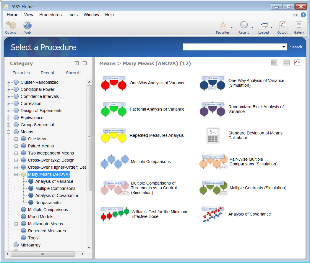
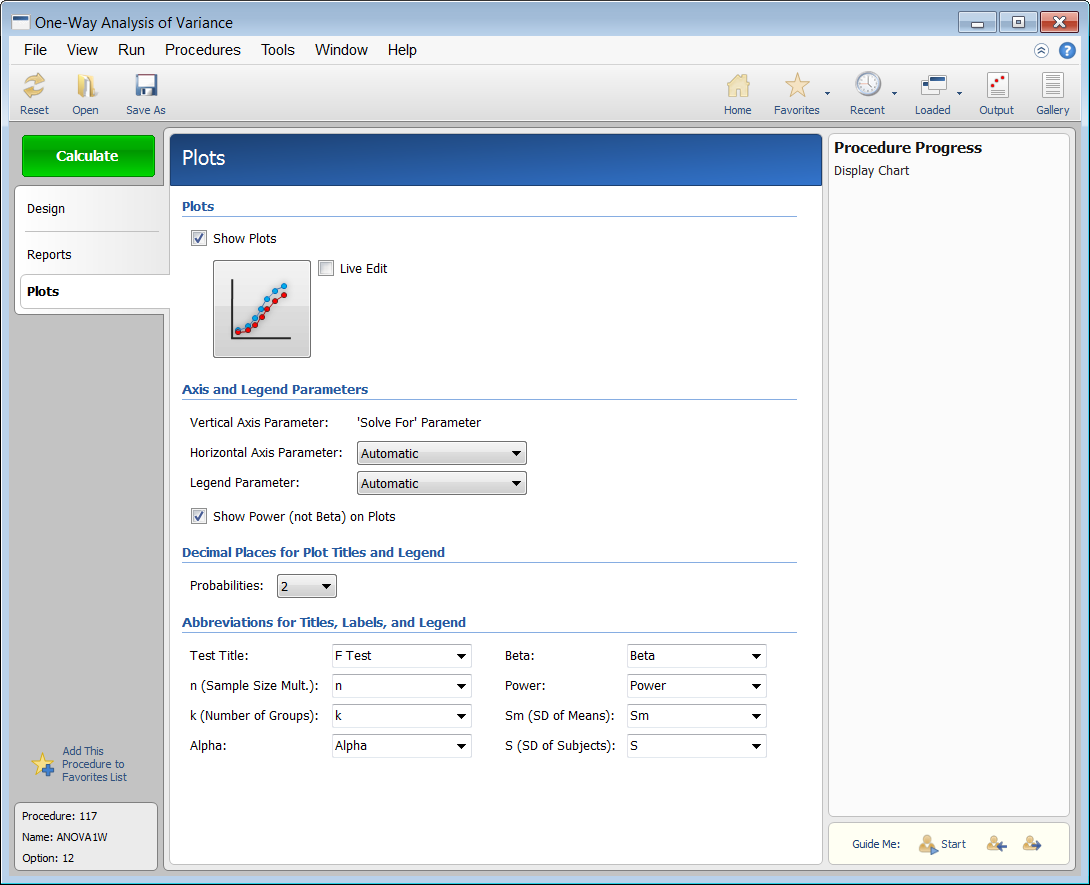
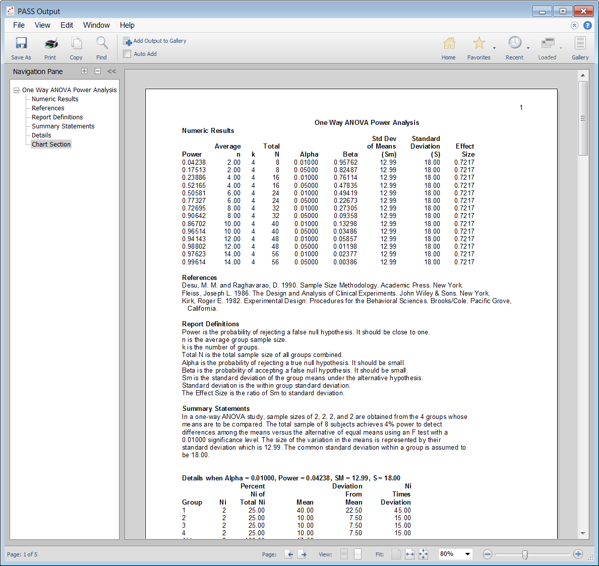
When the PASS software is first opened, the user is presented with the PASS Home window. From this window the desired procedure is selected from the menus, the category tree on the left, or with a procedure search. The procedure opens and the desired entries are made. When you click the Calculate button the results are produced. You can easily navigate to any part of the output with the navigation pane on the left.
PASS Home Window

Procedure Window for One-Way ANOVA

PASS Output Window

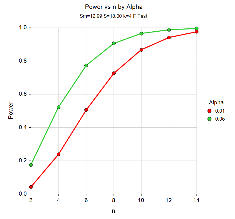
One-Way ANOVA Power Curve

Sample Size for One-Way Analysis of Variance
There are two procedures in PASS for sample size and power analysis of one-way analysis of variance studies. In one procedure the power and sample size calculations are made analytically, while in the other procedure, simulation is used. In both procedures, flexible sample size pattern options are included.
In the simulation procedure, the Kruskal-Wallis test may be analyzed, as well as the common one-way ANOVA F-test. A variety of underlying distributions for the groups may be simulated, including Beta, Binomial, Poisson, Gamma, Multinomial, Tukey's Lambda, Weibull, and Normal.
Sample Size for One-Way Analysis of Variance F-Tests using Effect Size
In our more advanced one-way ANOVA procedure, you are required to enter hypothesized means and variances. This simplified procedure only requires the input of an effect size, usually f, as proposed by Cohen (1988).
Sample Size for Factorial Analysis of Variance
This procedure performs power analysis and sample size estimation for an analysis of variance design with up to three fixed factors. Each factor may be specified to have any number of levels. Interaction term analysis may also be specified.
Sample Size for Factorial Analysis of Variance using Effect Size
This routine calculates power or sample size for F tests from a multi-factor analysis of variance design using only Cohen’s (1988) effect sizes as input.
Sample Size for Randomized Block Analysis of Variance
This procedure analyzes a randomized block analysis of variance with up to two treatment factors and the interaction. It provides tables of power values for various configurations of the randomized block design.
Sample Size for Repeated Measures Analysis
This procedure calculates the power for repeated measures designs having up to three between factors and up to three within factors. It computes power for both the univariate (F test and F test with Geisser-Greenhouse correction) and multivariate (Wilks’ lambda, Pillai-Bartlett trace, and Hotelling-Lawley trace) approaches. It can also be used to calculate the power of crossover designs.
Repeated measures designs are popular because they allow a subject to serve as their own control. This usually improves the precision of the experiment. However, when the analysis of the data uses the traditional F tests, additional assumptions concerning the structure of the error variance must be made. When these assumptions do not hold, the Geisser-Greenhouse correction provides reasonable adjustments so that significance levels are accurate.
An alternative to using the F test with repeated measures designs is to use one of the multivariate tests: Wilks’ lambda, Pillai-Bartlett trace, or Hotelling-Lawley trace. These alternatives are appealing because they do not make the strict, often unrealistic, assumptions about the structure of the variance-covariance matrix. Unfortunately, they may have less power than the F test and they cannot be used in all situations.
Sample Size for Multiple Comparisons
The following multiple comparisons procedures are available in PASS:
- Multiple Comparisons
- Pair-Wise Multiple Comparisons (Simulation)
- Multiple Comparisons of Treatments vs. a Control (Simulation)
- Multiple Contrasts (Simulation)
- Williams' Test for the Minimum Effective Dose
The analytic procedure for multiple comparisons considers three types of multiple comparison: all-pairs (Tukey-Kramer), with best (Hsu), and with control (Dunnett).
The three simulation procedures permit a variety of underlying distributions to be examined in terms of power and effective alpha. The sample-size needed for both any-pair, and all-pair power may be investigated in each of these procedures. For each scenario, two simulations are run: one estimates the significance level and the other estimates the power.
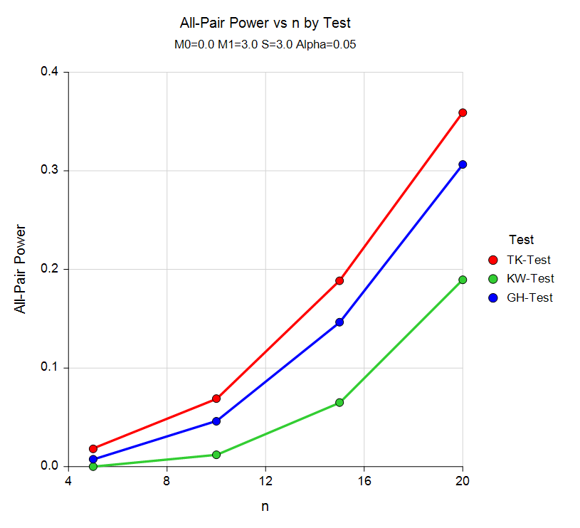
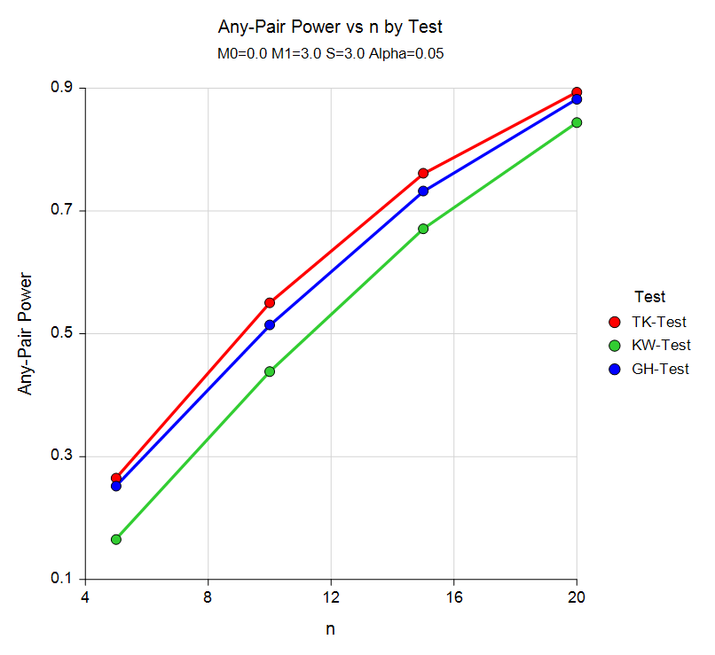
The Pair-Wise Multiple Comparisons (Simulation) procedure uses simulation analyze the power and significance level of three pair-wise multiple-comparison procedures: Tukey-Kramer, Kruskal-Wallis, and Games-Howell.
The Multiple Comparisons of Treatments vs. a Control (Simulation) procedure uses simulation to analyze the power and significance level of two multiple-comparison procedures that perform two-sided hypothesis tests of each treatment group mean versus the control group mean using simulation. These are Dunnett’s test and the Kruskal-Wallis test.
The Multiple Contrasts (Simulation) procedure uses simulation to analyze the power and significance level of two multiple-comparison procedures that perform two-sided hypothesis tests of contrasts of the group means. These are the Dunn-Bonferroni test and the Dunn-Welch test.
The Williams' Test for the Minimum Effective Dose procedure is used find the power or sample size for Williams' Test. The biological activity (i.e. toxicity) of a substance may be investigated by experiments in which the treatments are a series of monotonically increasing (or decreasing) doses of the substance. One of the aims of such a study is to determine the minimum effective dose (the lowest dose at which there is activity). Williams (1971, 1972) describes such a test. Chow et al. (2008) give the details of performing a power analysis and sample size calculation of this test.
Comparative All-Pair and Any-Pair Power Curves from the Pair-Wise Multiple Comparisons (Simulation) Procedure


Sample Size for Analysis of Covariance
Analysis of Covariance (ANCOVA) is an extension of the one-way analysis of variance model that adds quantitative variables (covariates). When used, it is assumed that their inclusion will reduce the size of the error variance and thus increase the power of the design.
We found two, slightly different, formulations for computing power for analysis of covariance. Keppel (1991) gives results that are based on a modification of the standard deviation by an amount proportional to the standard deviation reduction due to the covariate. Borm et al. (2007) give results that use a normal approximation to the noncentral F distribution. We use the Keppel approach in PASS.
Sample Size for Mixed Models
This procedure power analyzes random effects designs in which the outcome (response) is continuous. Thus, as with the analysis of variance (ANOVA), the procedure is used to test hypotheses comparing various group means. Unlike ANOVA, this procedure relaxes the strict assumptions regarding the variances of the groups. Random effects models are commonly used to analyze longitudinal (repeated measures) data.
This procedure extends many of the classical statistical techniques to the case when the variances are not equal, such as
- Two-sample designs (extending the t-test)
- One-way layout designs (extending one-way ANOVA)
- Factorial designs (extending factorial GLM)
- Split-plot designs (extending split-plot GLM)
- Repeated-measures designs (extending repeated-measures GLM)
- Cross-over designs (extending GLM)
Types of Linear Mixed Models
Several linear mixed model subtypes exist that are characterized by the random effects, fixed effects, and covariance structure they involve. These include fixed effects models, random effects models, and covariance pattern models.
Fixed Effects Models
A fixed effects model is a model where only fixed effects are included in the model. An effect (or factor) is fixed if the levels in the study represent all levels of interest of the factor, or at least all levels that are important for inference (e.g., treatment, dose, etc.). No random components are present. The general linear model is a fixed effects model. Fixed effects models can include interactions. The fixed effects can be estimated and tested using the F-test.
The fixed effects in the model include those factors for which means, standard errors, and confidence intervals will be estimated and tests of hypotheses will be performed. Other variables for which the model is to be adjusted (that are not important for estimation or hypothesis testing) can also be included in the model as fixed factors.
Random Effects Models
A random effects model includes both fixed and random terms in the model. An effect (or factor) is random if the levels of the factor represent a random subset of a larger group of levels (e.g., patients). The random effects are not tested, but are included to make the model more realistic.
Longitudinal Data Models
Longitudinal data arises when more than one response is measured on each subject in the study. Responses are often measured over time at fixed time points. A time point is fixed if it is pre-specified. Various variance-matrix structures can be employed to model the variance and correlation among repeated measurements.
Types of Factors
Between-Subject Factors
Between-subject factors are those that separate the experimental subjects into groups. If twelve subjects are randomly assigned to three treatment groups (four subjects per group), treatment is a between-subject factor.
Within-Subject Factors
Within-subject factors are those in which the response is measured on the same subject at several time points. Within-subject factors are those factors for which multiple levels of the factor are measured on the same subject. If each subject is measured at the low, medium, and high level of the treatment, treatment is a within-subject factor.
Sample Size for GEE Tests for Multiple Means in a Cluster-Randomized Design
This module calculates the power for testing for differences among the group means from continuous, correlated data from a cluster-randomized design that are analyzed using the GEE method.
GEE is different from mixed models in that it does not require the full specification of the joint distribution of the measurements, as long as the marginal mean model is correctly specified.
Estimation consistency is achieved even if the correlation matrix is incorrect. For clustered designs such as those discussed here, GEE assumes a compound symmetric (CS) correlation structure.
The outcomes are averaged at the cluster level. The precision of the experiment is increased by increasing the number of subjects per cluster as well as the number of clusters.
Sample Size for Multivariate Analysis of Variance (MANOVA)
This procedure calculates power for multivariate analysis of variance (MANOVA) designs having up to three factors. It computes power for three MANOVA test statistics: Wilks’ lambda, Pillai-Bartlett trace, and Hotelling-Lawley trace.
MANOVA is an extension of common analysis of variance (ANOVA). In ANOVA, differences among various group means on a single-response variable are studied. In MANOVA, the number of response variables is increased to two or more. The hypothesis concerns a comparison of vectors of group means. The multivariate extension of the F-test is not completely direct. Instead, several test statistics are available. The actual distributions of these statistics are difficult to calculate, so we rely on approximations based on the F-distribution.
Sample Size for Hotelling's T2
This procedure calculates power or sample size for Hotelling’s one-group, and two-group, T-squared (T2) test statistics. Hotelling’s T2 is an extension of the univariate t-tests in which the number of response variables is greater than one. In the two-group case, these results may also be obtained using PASS’s MANOVA test.
Sample Size for Multi-Arm versus a Control
In this design, there are k treatment groups and one control group. A mean is measured in each group. A total of k hypothesis tests are anticipated, each comparing a treatment group with the common control group using a test of the difference between two means. The Bonferroni adjustment of the type I error rate is used in these procedures.
