Sample Size for One or Two Means in PASS
PASS contains over 60 tools for sample size estimation and power analysis of the comparison of one, two, or paired means, including t-tests, equivalence, non-inferiority, cross-over, nonparametric, and simulation, among many others. Each procedure is easy-to-use and is carefully validated for accuracy. Use the links below to jump to a means topic. For each procedure, only a brief summary of the procedure is given. For more details about a particular procedure, we recommend you
download and install the free trial of the software.
Jump to:
Introduction
For most of the sample size procedures in PASS for comparing means, the user may choose to solve for sample size, power, or the population effect size in some manner. In the case of confidence intervals, one could solve for sample size or the distance to the confidence limit.
In a typical means test procedure where the goal is to estimate the sample size, the user enters power, alpha, desired population mean difference, and a value for the variation. The procedure is run and the output shows a summary of the entries as well as the sample size estimate. A summary statement is given, as well as references to the articles from which the formulas for the result were obtained.
For many of the parameters (e.g., power, alpha, sample size, means, standard deviations, etc.), multiple values may be entered in a single run. When this is done, estimates are made for every combination of entered values. A numeric summary of these is results is produced as well as easy-to-read sample size or power curve graphs.
Several simulation procedures are available for the comparison of means. These procedures can be used to examine the effects of non-normal underlying distributions, or to analyze sample size or power in scenarios where closed form solutions are not available.
Technical Details
This page provides a brief description of the tools that are available in PASS for power and sample size analysis of the comparison of means. If you would like to examine the formulas and technical details relating to a specific PASS procedure, we recommend you
download and install the free trial of the software, open the desired means procedure, and click on the help button in the top right corner to view the complete documentation of the procedure. There you will find summaries, formulas, references, discussions, technical details, examples, and validation against published articles for the procedure.
An Example Setup and Output
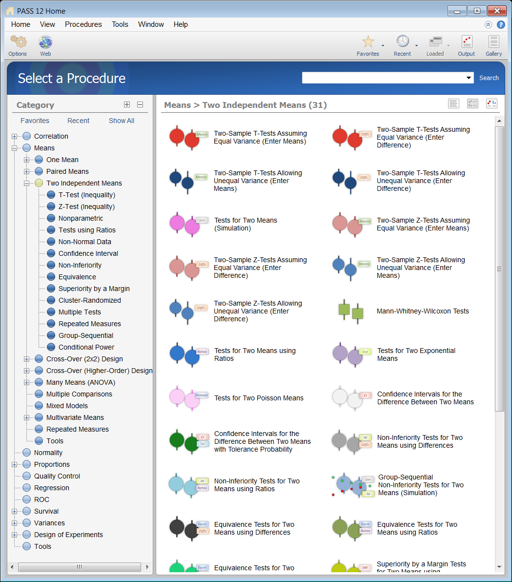
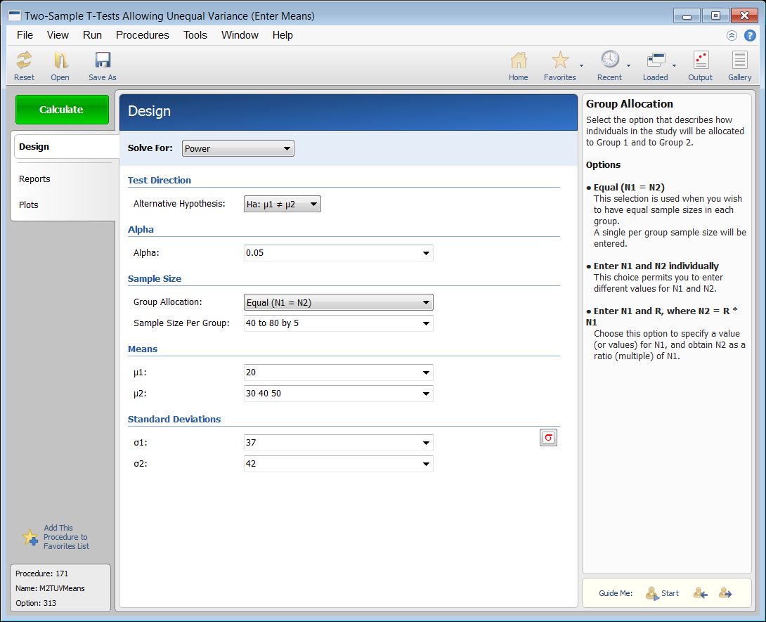
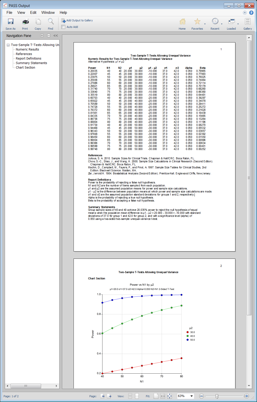
When the PASS software is first opened, the user is presented with the PASS Home window. From this window the desired procedure is selected from the menus, the category tree on the left, or with a procedure search. The procedure opens and the desired entries are made. When you click the Calculate button the results are produced. You can easily navigate to any part of the output with the navigation pane on the left.
PASS Home Window

Procedure Window for Two-Sample T-Tests

PASS Output Window

Sample Size for One Mean Tests and Confidence Intervals
Sample Size for Tests for One Mean
The one-sample t-test is used to test whether the mean of a population is greater than, less than, or not equal to a specific value. Because the t distribution is used to calculate critical values for the test, this test is often called the one-sample t-test. If the standard deviation is known, the normal distribution is used instead of the t distribution and the test is officially known as the z test.
This module also calculates the power of the nonparametric analog of the t-test, the Wilcoxon test.
Sample Size for Tests for One Mean (Simulation)
This procedure allows you to study the power and sample size of several statistical tests of the hypothesis that the population mean is equal to a specific value versus the alternative that it is greater than, less than, or not equal to that value. The one-sample t-test is commonly used in this situation, but other tests have been developed for situations where the data are not normally distributed. These additional tests include the Wilcoxon signed-rank test, the sign test, and the computer-intensive bootstrap test. When the population follows the exponential distribution, a test based on this distribution should be used.
The t-test assumes that the data are normally distributed. When this assumption does not hold, the t-test is still often used, hoping that its robustness will produce accurate results. This procedure allows you to study the accuracy of various tests using simulation techniques. A wide variety of distributions can be simulated to allow you to assess the impact of various forms of non-normality on each test’s accuracy.
Sample Size for Tests for One Mean using Effect Size
This procedure provides sample size and power calculations for a one- or two-sided one-sample t-test when the effect size is specified rather than the means and variance, as described by Cohen (1988). In this design, a single population of independent, normally distributed data is sampled and its mean is compared to a specified quantity by forming the difference scaled by the standard deviation.
Sample Size for Tests for One Exponential Mean
This procedure analyzes studies for testing hypotheses about the mean of the exponential distribution. Such tests are often used in reliability acceptance testing, also called reliability demonstration testing.
Results are calculated for plans that are time censored or failure censored, as well as for plans that use with replacement or without replacement sampling. We adopt the basic methodology outlined in Epstein (1960), Juran (1979), Bain and Engelhardt (1991), and Schilling (1982).
Sample Size for Tests for One Poisson Mean
The Poisson probability law gives the probability distribution of the number of events occurring in a specified interval of time or space. The Poisson distribution is often used to fit count data, such as the number of defects on an item, the number of accidents at an intersection during a year, the number of calls to a call center during an hour, or the number of meteors seen in the evening sky during an hour.
The Poisson distribution is characterized by a single parameter, λ, which is the mean number of occurrences during the interval. This procedure calculates the power or sample size for testing whether λ is less than or greater than a specified value. This test is usually called the test of the Poisson mean.
The test is described in Ostle (1988) and the power calculation is given in Guenther (1977).
Sample Size for Non-Inferiority Tests for One Mean
This module computes power and sample size for non-inferiority tests in one-sample designs in which the outcome is distributed as a normal random variable. Sample size formulas for non-inferiority tests of a single mean are presented in Chow et al. (2003) page 50. This module also calculates the power of the nonparametric analog of the t-test, the Wilcoxon test.
Sample Size for Superiority by a Margin Tests for One Mean
This module computes power and sample size for tests in one-sample designs with a superiority margin in which the outcome is distributed as a normal random variable. Sample size formulas for non-inferiority and superiority hypothesis tests of a single mean are presented in Chow et al. (2003) page 50. This module also calculates the power of the non-parametric analog of the t-test, the Wilcoxon test.
Sample Size for Multiple One-Sample T-Tests
This procedure analyzes power and sample size (number of arrays) for paired and one sample high-throughput studies. False discovery rate and experiment-wise error rate control methods are available in this procedure. Values that can be varied in this procedure are power, false discovery rate and experiment-wise error rate, sample size (number of arrays), the minimum mean difference detected, the standard deviation, and in the case of false discovery rate control, the number of genes with minimum mean difference.
Sample Size for Conditional Power of One-Sample T-Tests
In sequential designs, one or more intermediate analyses of the emerging data are conducted to evaluate whether the experiment should be continued. This may be done to conserve resources or to allow a data monitoring board to evaluate safety and efficacy when subjects are entered in a staggered fashion over a long period of time. Conditional power (a frequentist concept) is the probability that the final result will be significant, given the data obtained up to the time of the interim look. Predictive power (a Bayesian concept) is the result of averaging the conditional power over the posterior distribution of effect size. Both of these methods fall under the heading of stochastic curtailment techniques. Further reading about the theory of these methods can be found in Chow and Chang (2007), Chang (2008, 2008), Proschan et. al (2006), and Dmitrienko et. al (2005).
This program module computes conditional and predicted power for the case when a one-sample t-test is used to test whether the mean of a population is greater than, less than, or not equal to a specific value.
Conditional power procedures are also available for the case of Non-Inferiority and Superiority by a Margin.
Sample Size for Group-Sequential Tests for One Mean with Known Variance (Simulation)
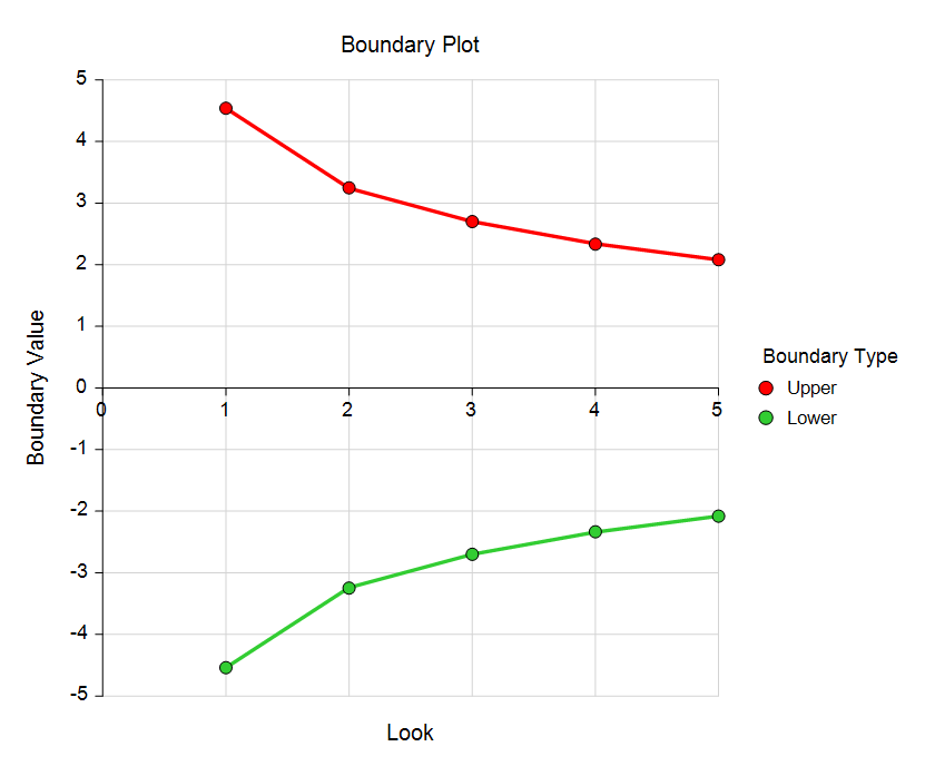
This procedure can be used to determine power, sample size and/or boundaries for group-sequential tests comparing a mean with a known standard deviation to a hypothesized mean. The underlying test is the common, known-variance one-sample Z-test. For one- and two-sided tests, efficacy and/or futility boundaries can be generated. The spacing of the stages can be equal or custom specified. Individual stages may also be skipped. Boundaries can be computed based on popular alpha- and beta-spending functions (O’Brien-Fleming Analog, Pocock Analog, Hwang-Shih-DeCani Gamma family, linear) or custom spending functions, or boundaries may be input directly, if desired. Futility boundaries can be binding or non-binding. Corresponding P-Value boundaries are given for each boundary statistic. Alpha and/or beta spent at each stage is reported. Plots of boundaries are also produced.
This procedure is used as the planning tool for determining sample size and initial boundaries. Stage data, as it is obtained, can be evaluated using the companion procedure, Group-Sequential Analysis for One Mean with Known Variance, found in NCSS software. The companion procedure also gives the option for sample-size re-estimation and updated boundaries for current-stage information. In that procedure, simulation can be used to evaluate boundary-crossing probabilities given the current stage results.
Sample Size for Group-Sequential T-Tests for One Mean (Simulation)
This procedure can be used to determine power, sample size and/or boundaries for group-sequential t-tests comparing a single mean to a hypothesized mean.
Stage data, as it is obtained, can be evaluated using the companion procedure Group-Sequential T-Tests for One Mean. The companion procedure also gives the option for sample-size re-estimation and updated boundaries for current-stage information.
Sample Size for Confidence Intervals for One Mean
This procedure calculates the sample size necessary to achieve a specified distance from the mean to the confidence limit(s) at a stated confidence level for a confidence interval about the mean when the underlying data distribution is normal.
This procedure assumes that the standard deviation of the future sample will be the same as the standard deviation that is specified. If the standard deviation to be used in the procedure is estimated from a previous sample or represents the population standard deviation, the Confidence Intervals for One Mean with Tolerance Probability procedure should be considered. That procedure controls the probability that the distance from the mean to the confidence limits will be less than or equal to the value specified.
Sample Size for Confidence Intervals for One Mean with Tolerance Probability
This procedure calculates the sample size necessary to achieve a specified distance from the mean to the confidence limit(s) with a given tolerance probability at a stated confidence level for a confidence interval about a single mean when the underlying data distribution is normal.
Sample Size for Confidence Intervals for One Mean in a Stratified Design
This procedure calculates sample size and half-width for confidence intervals of a mean from a stratified design in which the outcome variable is continuous. It uses the results from elementary sampling theory which are presented in many works including Yamane (1967) and Levy and Lemeshow (2008).
Suppose that the mean of a continuous outcome variable of a sample from a population of subjects (or items) is to be estimated with a confidence interval. Further suppose that the population can be separated into a few subpopulations, often called strata. If these strata are created so that items are similar within a particular stratum, but quite different between strata, then a stratified design might be adopted for a number of reasons. Note that the population may be finite or infinite.
This procedure allows you to determine the appropriate sample size to be taken from each stratum so that various parameters of the confidence interval are guaranteed. These parameters include the confidence level and width of the interval.
Sample Size for Confidence Intervals for One Mean in a Cluster-Randomized Design
This procedure calculates sample size and half-width for confidence intervals of a mean from a cluster-randomized design in which the outcome variable is continuous. It uses the results from Ahn, Heo, and Zang (2015), Lohr (2019), and Campbell and Walters (2014).
Suppose that the mean of a continuous outcome variable of a sample from a population of subjects (or items) is to be estimated with a confidence interval. Further suppose that the population is separated into small groups, called clusters. These clusters may contain different numbers of items.
This procedure allows you to determine the appropriate number of clusters to be sampled so that the width of a confidence interval of the mean may be guaranteed at a certain confidence level.
Sample Size for Confidence Intervals for One Mean in a Stratified Cluster-Randomized Design
This procedure calculates sample size and half-width for confidence intervals of a mean from a stratified cluster randomization trial (CRT) in which the outcome variable is continuous. It uses the results from elementary sampling theory which are presented in Wang, Zhang, and Ahn (2017) and Xu, Zhu, and Ahn (2019).
Suppose that the mean of a continuous outcome variable of a sample from a population of subjects (or items) is to be estimated with a confidence interval. Further suppose that the population can be separated into a few subpopulations, often called strata. Further suppose that each stratum can be separated into a number of clusters and that sampling occurs at the cluster level. That is, a simple random sample of clusters is drawn within a stratum. Next, a simple random sample of subjects is drawn from within each cluster.
Note that this procedure assumes an infinite population in which the size of every cluster and every stratum is not know.
This procedure allows you to determine the appropriate sample size to be taken from each stratum so that width of the confidence interval is guaranteed.
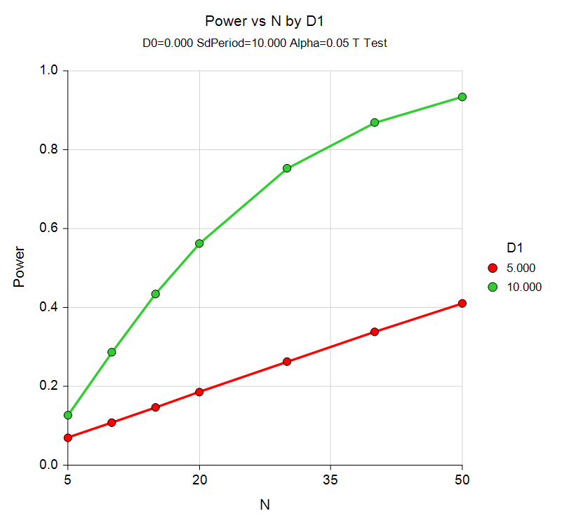
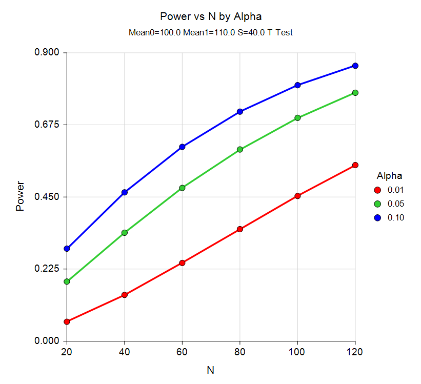
Power Curve from the Tests for One Mean Procedure

Sample Size for Paired Means Tests and Confidence Intervals
Sample Size for Tests for Paired Means
The paired t-test may be used to test whether the mean difference of two populations is greater than, less than, or not equal to a specific value. This procedure calculates sample size or power of a study based on the specified mean and standard deviation of paired differences.
This module also calculates the power of the nonparametric analog of the t-test, the Wilcoxon test.
Sample Size for Tests for Paired Means (Simulation)
This procedure allows you to study the power and sample size of several statistical tests of the null hypothesis that the difference between two correlated means is equal to a specific value versus the alternative that it is greater than, less than, or not-equal to that value. The paired t-test is commonly used in this situation. Other tests have been developed for the case when the data are not normally distributed. These additional tests include the Wilcoxon signed-ranks test, the sign test, and the computer-intensive bootstrap test.
Paired data may occur because two measurements are made on the same subject or because measurements are made on two subjects that have been matched according to other, often demographic, variables. Hypothesis tests on paired data can be analyzed by considering the differences between the paired items. The distribution of differences is usually symmetric. Thus, the paired t-test and the Wilcoxon signed-rank test are often appropriate for paired data even when the distributions of the individual items are not normal.
Sample Size for Tests for Paired Means using Effect Size
This procedure provides sample size and power calculations for a one- or two-sided paired t-test when the effect size is specified rather than the means and variance, as described in Cohen (1988). In this design, a single population of paired, normally distributed data is sampled and the mean difference is compared to zero by forming the difference scaled by the standard deviation of the differences.
Sample Size for Tests for the Matched-Pair Difference of Two Means in a Cluster-Randomized Design
Cluster-randomized designs are those in which whole clusters of subjects (classes, hospitals, communities, etc.) are sampled, rather than individual subjects. This sample size and power procedure is used for the case where the subject responses are continuous (mean outcome). To reduce the variation (and thus increase power), clusters are matched, with one cluster of each pair assigned to the control group, and the other assigned the treatment group. This procedure gives the number of pairs needed for the desired power requirement.
Sample Size for Non-Inferiority Tests for Paired Means
This module computes power and sample size for non-inferiority tests in paired designs in which the outcome difference is distributed as a normal random variable. Sample size formulas for non-inferiority tests of a single mean (and hence paired differences) are presented in Chow et al. (2003) page 50. This module also calculates the power of the nonparametric analog of the t-test, the Wilcoxon test.
Sample Size for Superiority by a Margin Tests for Paired Means
This module computes power and sample size for tests in paired-sample designs with a superiority margin in which the outcome difference is distributed as a normal random variable. Sample size formulas for non-inferiority and superiority hypothesis tests of a single mean are presented in Chow et al. (2003) page 50. This module also calculates the power of the non-parametric analog of the t-test, the Wilcoxon test.
Sample Size for Equivalence Tests for Paired Means (Simulation)
This procedure allows you to study the power and sample size of tests of equivalence of means of two correlated variables. Schuirmann’s (1987) two one-sided tests (TOST) approach is used to test equivalence. The paired t-test is commonly used in this situation. Other tests have been developed for the case when the data are not normally distributed. These additional tests include the Wilcoxon signed-ranks test, the sign test, and the computer-intensive bootstrap test.
Sample Size for Conditional Power of Paired T-Tests
This procedure computes conditional and predicted power for the case when a paired t-test is used to test whether the paired mean difference is greater than, less than, or not equal to a specific value.
In PASS, conditional power procedures are also available for the case of Non-Inferiority and Superiority by a Margin.
Sample Size for Multiple Paired T-Tests
This procedure estimates power and sample size (number of arrays) for paired and one sample high-throughput studies. False discovery rate and experiment-wise error rate control methods are available in this procedure. Values that can be varied in this procedure are power, false discovery rate and experiment-wise error rate, sample size (number of arrays), the minimum mean difference detected, the standard deviation, and in the case of false discovery rate control, the number of genes with minimum mean difference.
Sample Size for Confidence Intervals for Paired Means
This procedure calculates the sample size necessary to achieve a specified distance from the paired sample mean difference to the confidence limit(s) at a stated confidence level for a confidence interval about the mean difference when the underlying data distribution is normal.
Sample Size for Confidence Intervals for Paired Means with Tolerance Probability
This procedure calculates the sample size necessary to achieve a specified distance from the paired sample mean difference to the confidence limit(s) with a given tolerance probability at a stated confidence level for a confidence interval about a single mean difference when the underlying data distribution is normal.
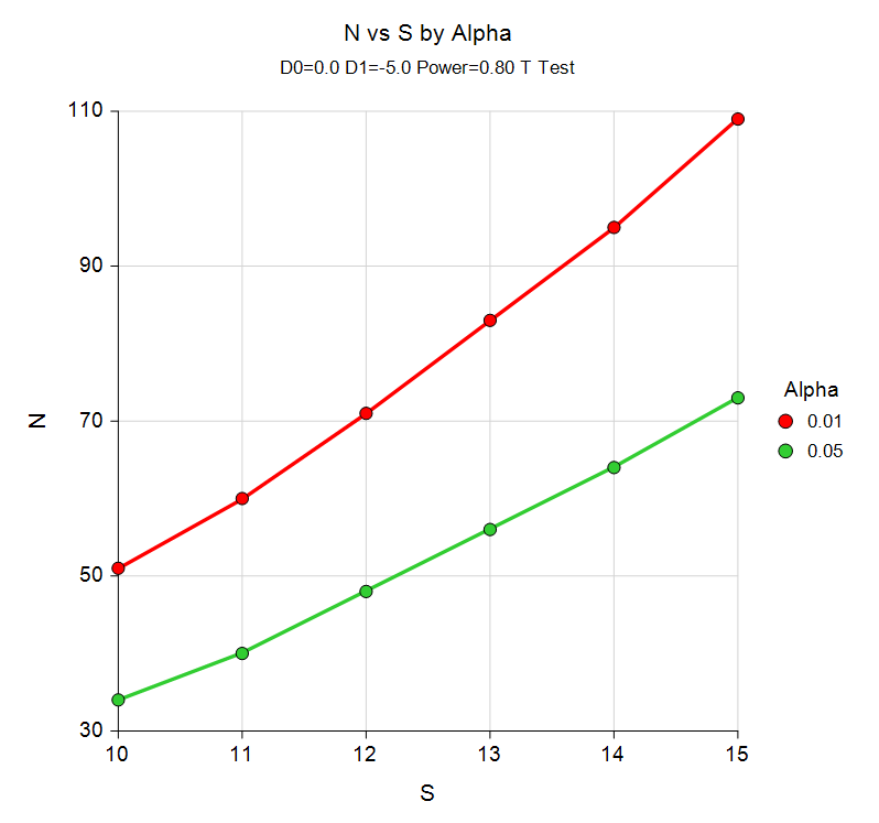
Sample Size Curve from the Tests for Paired Means Procedure

Sample Size for Two Independent Means Tests and Confidence Intervals
Sample Size for T-Test (Inequality)
There are five procedures in PASS for the comparison of two means using t-tests. Two of the procedures (enter means and enter mean difference) assume equal variance and use the standard t-test formulas. Two more of the procedures (enter means and enter mean difference) assume the variances are unequal and use formulas based on Welch's unequal variance t-test. The fifth procedure uses simulation to determine the effect of various underlying distributions on the sample size or power result.
For each of the procedures, one-sided or two-sided test options are available, as well as equal or unequal sample sizes in the two groups.
Sample Size for Two-Sample T-Tests using Effect Size
This procedure provides sample size and power calculations for one- or two-sided two-sample t-tests when the effect size is specified rather than the means and variance(s), as described in Cohen (1988). The design corresponding to this test procedure is sometimes referred to as a parallel-groups design. In this design, two groups from independent, normally distributed populations are compared by considering the difference in their means scaled be their common standard deviation.
This procedure is specific to the two-sample t-test assuming equal variance. If the variances are known to be significantly different, this procedure can still be used if the group sample sizes are equal and the average of the variances is used.
Sample Size for Z-Test (Inequality)
There are four procedures in PASS for the comparison of two means using z-tests. Two of the procedures (enter means and enter mean difference) assume equal variance and use the corresponding z-test formulas. Two more of the procedures (enter means and enter mean difference) assume the variances are unequal. For each of the procedures, one-sided or two-sided test options are available, as well as equal or unequal sample sizes in the two groups.
Sample Size for Nonparametric Tests of Two Independent Means
This procedure uses simulation to determine the power or sample size for the Mann-Whitney-Wilcoxon test. Some of the available distributions include Beta, Normal, Multinomial, Weibull, Tukey's Lambda, Gamma, and Normal.
Sample Size for Tests of Two Independent Means Using Ratios
This procedure calculates power and sample size for t-tests from a parallel-groups design in which the logarithm of the outcome is a continuous normal random variable. This routine deals with the case in which the statistical hypotheses are expressed in terms of mean ratios instead of mean differences.
Sample Size for Tests of Two Independent Means with Non-Normal Data
PASS has specific tools for the calculation of sample sizes or power for the case where the compared means are based on samples from a Poisson distribution or an exponential distribution. There are also two simulation procedures for t-tests and Mann-Whitney-Wilcoxon tests where the underlying distribution can be specified directly.
Sample Size for Confidence Intervals for Comparing Two Independent Means
Two confidence interval procedures can be used in PASS to calculate sample size for a given distance from the mean difference to the confidence interval limits. One procedure has the additional option of accounting for the variability in a future estimate of the pooled standard deviation through a tolerance probability.
Sample Size for Non-Inferiority Tests of Two Independent Means
One procedure examines power and sample size for non-inferiority of two independent means based on the difference, while the other procedure is based on the mean ratio. There is also a group-sequential non-inferiority test procedure.
Sample Size for Equivalence Tests of Two Independent Means
There are three equivalence test procedures in PASS. One procedure is based on mean differences, another on the ratios, and the third is a simulation based procedure with options for t-tests, Mann-Whitney-Wilcoxon tests, and trimmed mean tests.
Sample Size for Equivalence Tests for the Ratio of Two Means (Normal Data)
This procedure calculates power and sample size of statistical tests for equivalence tests from parallel-group design with two groups when the data are assumed to follow the normal distribution (so the log transformation is not used). This routine deals with the case in which the statistical hypotheses are expressed in terms of mean ratios rather than mean differences.
The details of this analysis are given in Hauschke et al. (1999) and Kieser and Hauschke (1999).
Note that when the data follow a log-normal distribution rather than the normal distribution, you should use another PASS procedure entitled Equivalence Tests for the Ratio of Two Means (Log-Normal Data) to obtain more accurate results.
Sample Size for Superiority by a Margin Tests of Two Independent Means
These two procedures in PASS are used when one wishes to calculate sample size or power for the case of showing one group mean is higher (or lower) than another by a specified amount.
Sample Size for Cluster-Randomized Tests of Two Independent Means
In this procedure, cluster randomization refers to the situation in which the means of two groups, made up of M clusters of N individuals each, are to be tested using a modified t-test. This procedure permits the user to solve for the power, the number of clusters, or the number of individuals within a cluster.
Sample Size for Mixed Models Tests for Two Means in a Cluster-Randomized Design
This procedure calculates power and sample size for a two-level hierarchical mixed model in which clusters (groups, classes, hospitals, etc.) of subjects are measured one time (cross-sectional) on a continuous variable. The goal of the study is to compare the two group means.
In this design, the subjects are the level one units and the clusters are the level two units. All subjects in a particular cluster (level two unit) receive one of two possible interventions. This intervention is selected at random. Note that a companion procedure power analyzes the other case in which the randomization occurs for the level one units (the subjects).
Note that this procedure provides results for fixed cluster sizes. Another procedure provides results for variable cluster sizes.
Sample Size for Tests for Two Means in a Stepped-Wedge Cluster-Randomized Design
A stepped-wedge cluster-randomized design is similar to a cross-over design in that each cluster receives both the treatment and control over time. In a stepped-wedge design, however, the clusters switch or cross-over in one direction only (usually from the control group to the treatment group). Once a cluster is randomized to the treatment group, it continues to receive the treatment for the duration of the study. In a typical stepped-wedge design the all clusters are assigned to the control group at the first time point and then individual clusters are progressively randomized to the treatment group over time. The stepped-wedge design is particularly useful for cases where it is logistically impractical to apply a particular treatment to half of the clusters at the same time.
This procedure computes power and sample size for tests for the difference between two means in cross-sectional stepped-wedge cluster-randomized designs. In cross-sectional designs, different subjects are measured within each cluster at each point in time. No one subject is measured more than once. (This is not to be confused with cohort studies (i.e. repeated measures) where individuals are measured at each point in time. The methods in this procedure should not be used for cohort or repeated measures designs.)
Sample Size for Mixed Models Tests for Two Means in a 2-Level Hierarchical Design (Level-2
Randomization)
This procedure calculates power and sample size for a two-level hierarchical mixed model in which clusters
(groups, classes, hospitals, etc.) of subjects are measured one time (cross-sectional) on a continuous variable. The
goal of the study is to compare the two group means.
In this design, the subjects are the level one units and the clusters are the level two units. All subjects in a
particular cluster (level two unit) receive one of two possible interventions. This intervention is selected at
random. Note that a companion procedure power analyzes the other case in which the randomization occurs for
the level one units (the subjects).
Sample Size for Mixed Models Tests for Two Means in a 2-Level Hierarchical Design (Level-1 Randomization)
This procedure calculates power and sample size for a two-level hierarchical mixed model in which clusters
(groups, classes, hospitals, etc.) of subjects are measured one time (cross-sectional) on a continuous variable. The
goal of the study is to compare the two group means.
In this design, the subjects are the level one units and the clusters are the level two units. Each subject in a
particular cluster (level two unit) is randomized individually to one of two possible interventions. Note that a
companion procedure power analyzes the other case in which the randomization occurs for the level two units (the
clusters).
Sample Size for Mixed Models Tests for Two Means at the End of Follow-Up in a 2-Level Hierarchical Design
This procedure calculates power and sample size for a two-level longitudinal design in which subjects (level-two
unit) are randomly assigned to one of two groups. Each subject is measured at several time points and the goal of
the study is to compare the group means of at the final time point. This procedure assumes that the group means
are identical at the beginning of the study (which they often are in a randomized trial).
All subjects in a group are assumed to have a common (fixed) slope. Each subject is assigned to receive one of
two possible interventions.
Sample Size for Mixed Models Tests for Two Means at the End of Follow-Up in a 3-Level Hierarchical Design (Level-3 Randomization)
This procedure calculates power and sample size for a three-level hierarchical design which is randomized at the
third level. Each subject (level-2 unit) is measured at several time points (level-1 units) and the goal of the study
is to compare the group means of at the final time point, i.e., at the end of follow-up.
The study is assumed to be longitudinal, so repeated measurements (level-1 units) are nested in patients (level-2
units) which are nested in clinics (level-3 units).
Each clinic (level-3 unit) is randomized into one of two intervention groups; e.g., treatment and control.
Sample Size for GEE Tests for Two Means in a Cluster-Randomized Design
This module calculates the power for testing the difference between two means obtained from a clusterrandomized
design. The mean come from continuous, correlated data that are analyzed using the GEE method.
Such data occur in two design types: clustered and longitudinal. This procedure is specific to cluster-randomized
designs. A companion procedure power analyzes data from a repeated measures design.
GEE is different from mixed models in that it does not require the full specification of the joint distribution of the
clustered measurements, as long as the marginal mean model is correctly specified. Estimation consistency is
achieved even if the correlation matrix is incorrect. Also, the correlation matrix of the responses is specified
directly, rather than using an intermediate, random effects model as is the case in mixed models. For clustered
designs, GEE often uses a compound symmetric (CS) correlation structure.
Time-averaged difference analysis is often used when the outcome varies with time. However, in this case, the
observations are treated as if they were repeated measurements from a subject (cluster). Each cluster is
randomized either in the treatment or the control group.
Making these assumptions, the data may be analyzed using the GEE TAD methodology. This procedure performs
a power analysis and sample size calculation for data obtained and analyzed in this manner.
Sample Size for GEE Tests for Two Means in a Stratified Cluster-Randomized Design
This procedure calculates power and sample size for tests of two means in a stratified cluster-randomized design
in which the outcome variable is continuous. It uses the work of Wang, Zhang, and Ahn (2017) which give the
power in a size-stratified cluster-randomized design in which the cluster size is allowed to vary within strata. The
analysis is of a simple means model fit with the GEE method.
Sample Size for Tests for Two Means in a Split-Mouth Design
This procedure assumes that continuous data will be obtained from a study that uses a split-mouth design. The GEE method is used to analyze the repeated measures model that is assumed. The sample size formula is derived in Zhu, Zhang, and Ahn (2017).
A split-mouth design is used in dental trials in which treatments are randomized over segments of the mouth within each subject. In this design, the mouth is divided into two or more segments or regions. For example, the segments might be top and bottom, left and right, or a combination of both. Within each segment, specific sites (e.g. teeth) are identified. The same treatment is applied to all sites within a segment.
The split-mouth design, also called the split-cluster design, is occasionally used in other areas such as dermatology and animal studies. Although the design may be used in other experiments, the terminology of the split-mouth design will be used in this procedure.
Sample Size for Multiple Tests of Two Independent Means
This procedure estimates power and sample size (number of arrays) for 2 group (two-sample) high-throughput studies. False discovery rate and experiment-wise error rate control methods are available in this procedure. Values that can be varied in this procedure are power, false discovery rate and experiment-wise error rate, sample sizes (numbers of arrays) in each group, the minimum mean difference detected, the standard deviations in each group, and in the case of false discovery rate control, the number of tests/genes with minimum mean difference.
Sample Size for Repeated Measures Tests of Two Independent Means
There are two repeated measures procedures for the comparison of two independent means. One of the procedures calculates the power for testing the time-averaged difference (TAD) between two means in a repeated measures design. The other procedure is used for the scenario of comparing two groups of pre-post scores.
Time-averaged difference analysis is often used when the outcome to be measured varies with time. The precision of the experiment is increased by taking multiple measurements from each individual and comparing the time-averaged difference between the two groups. Care must be taken in the analysis because of the correlation that is introduced when several measurements are taken from the same individual. The covariance structure may take on several forms depending on the nature of the experiment and the subjects involved. This procedure allows you to calculate sample sizes using four different covariance patterns: Compound Symmetry, AR(1), Banded(1), and Simple. This procedure can be used to calculate sample size and power for tests of pairwise contrasts in a mixed models analysis of repeated measures data.
The Tests for Two Groups of Pre-Post Scores procedure calculates the power for testing the interaction in a 2-by-2 repeated measures design. This particular repeated measures design is one in which subjects are observed twice over time, as is the case in a pre, post design. Measurements are taken at two, pre-determined time intervals. It is important that the time interval remains constant from subject to subject. The test of the interaction compares the average change in measurement for group 1 with that of group 2.
Sample Size for Group-Sequential Tests of Two Independent Means
There are four procedures in PASS for the comparison of two means with group-sequential tests. One of the procedures uses an analytic solution, but is much less flexible than the others. Two simulation procedures allow for various underlying distributions. The fourth uses simulation for non-inferiority group-sequential testing.
A variety of spending function options are available in these procedures, including Hwang-Shi-DeCani, O'Brien-Fleming, and Pocock types. Either the T-test or the Mann-Whitney-Wilcoxon test may be examined. For one-sided tests, significance and futility boundaries can be produced. The spacing of the looks can be equal or custom specified. The distributions of each of the groups under the null and alternative hypotheses can be specified directly using over ten distributions including normal, exponential, Gamma, Uniform, Beta, and Cauchy. Boundaries can also be input directly to verify alpha- and/or beta-spending properties. Futility boundaries can be binding or non-binding.

Sample Size for Group-Sequential Tests for Two Means with Known Variances (Simulation)
This procedure can be used to determine power, sample size and/or boundaries for group-sequential tests comparing the means of two groups with known standard deviations. The underlying test is the common, known-variance two-sample Z-test. For one- and two-sided tests, efficacy and/or futility boundaries can be generated. The spacing of the stages can be equal or custom specified. Individual stages may also be skipped. Boundaries can be computed based on popular alpha- and beta-spending functions (O’Brien-Fleming Analog, Pocock Analog, Hwang-Shih-DeCani Gamma family, linear) or custom spending functions, or boundaries may be input directly, if desired. Futility boundaries can be binding or non-binding. Corresponding P-Value boundaries are given for each boundary statistic. Alpha and/or beta spent at each stage is reported. Plots of boundaries are also produced.
This procedure is used as the planning tool for determining sample size and initial boundaries. Stage data, as it is obtained, can be evaluated using the companion procedure Group-Sequential Analysis for Two Means with Known Variances. The companion procedure also gives the option for sample-size re-estimation and updated boundaries for current-stage information. In that procedure, simulation can be used to evaluate boundary-crossing probabilities given the current stage results.
Sample Size for Group-Sequential Non-Inferiority Tests for Two Means with Known Variances (Simulation)
This procedure can be used to determine power, sample size and/or boundaries for group-sequential non-inferiority tests comparing the means of two groups with known standard deviations. The underlying test is the common, known-variance two-sample Z-test, with a non-inferiority margin.
Stage data, as it is obtained, can be evaluated using the companion procedure Group-Sequential Non-Inferiority Analysis for Two Means with Known Variances. The companion procedure also gives the option for sample-size re-estimation and updated boundaries for current-stage information.
Sample Size for Group-Sequential Superiority by a Margin Tests for Two Means with Known Variances (Simulation)
This procedure can be used to determine power, sample size and/or boundaries for group-sequential superiority by a margin tests comparing the means of two groups with known standard deviations. The underlying test is the common, known-variance two-sample Z-test, with a superiority margin.
Stage data, as it is obtained, can be evaluated using the companion procedure Group-Sequential Superiority by a Margin Analysis for Two Means with Known Variances.
Sample Size for Group-Sequential T-Tests for Two Means (Simulation)
This procedure can be used to determine power, sample size and/or boundaries for group-sequential tests comparing the means of two groups using Welch’s t-test. For one- and two-sided tests, efficacy and/or futility boundaries can be generated. The spacing of the stages can be equal or custom specified. Individual stages may also be skipped. Boundaries can be computed based on popular alpha- and beta-spending functions (O’Brien-Fleming Analog, Pocock Analog, Hwang-Shih-DeCani Gamma family, linear) or custom spending functions, or boundaries may be input directly, if desired. Futility boundaries can be binding or non-binding. Corresponding P-Value boundaries are given for each boundary statistic (unless boundaries are input directly). Alpha and/or beta spent at each stage is reported. Plots of boundaries are also produced.
This procedure is used as the planning tool for determining sample size and initial boundaries. Stage data, as it is obtained, can be evaluated using the companion procedure Group-Sequential T-Tests for Two Means. The companion procedure also gives the option for sample-size re-estimation and updated boundaries for current-stage information. In that procedure, simulation can be used to evaluate boundary-crossing probabilities given the current stage results.
Sample Size for Group-Sequential Non-Inferiority T-Tests for Two Means (Simulation)
This procedure can be used to determine power, sample size and/or boundaries for group-sequential tests comparing the means of two groups using Welch’s t-test, with a non-inferiority margin.
Stage data, as it is obtained, can be evaluated using the companion procedure Group-Sequential Non-Inferiority T-Tests for Two Means.
Sample Size for Group-Sequential Superiority by a Margin T-Tests for Two Means (Simulation)
This procedure can be used to determine power, sample size and/or boundaries for group-sequential tests comparing the means of two groups using Welch’s t-test, with a superiority margin.
Stage data, as it is obtained, can be evaluated using the companion procedure Group-Sequential Superiority by a Margin T-Tests for Two Means.
Sample Size for Conditional Power Tests of Two Independent Means
The Conditional Power of Two-Sample T-Tests procedure computes conditional and predicted power for the case when a two-sample t-test is used to test whether the means of two populations are different.
In sequential designs, one or more intermediate analyses of the emerging data are conducted to evaluate whether the experiment should be continued. This may be done to conserve resources or to allow a data monitoring board to evaluate safety and efficacy when subjects are entered in a staggered fashion over a long period of time. Conditional power is the probability that the final result will be significant, given the data obtained up to the time of the interim look. Predictive power is the result of averaging the conditional power over the posterior distribution of effect size. Both of these methods fall under the heading of stochastic curtailment techniques.
Procedures are also available in PASS for the case of Non-Inferiority and Superiority by a Margin.
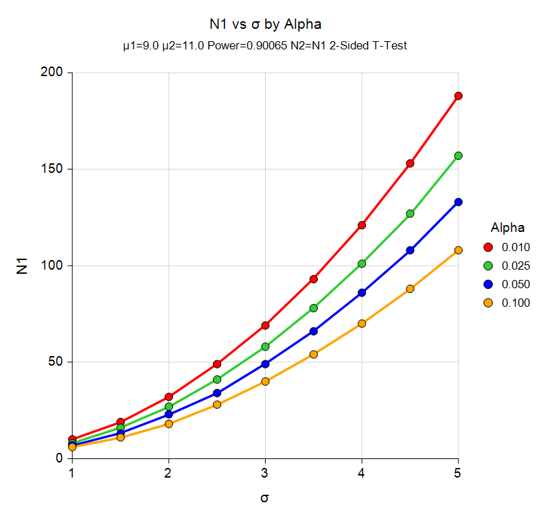
Sample Size Curve from the Two-Sample T-Tests Assuming Equal Variance (Enter Means) Procedure

Sample Size for Comparing Two Means in a Cross-Over Design
Sample Size for Tests for Two Means in a Cross-Over Design
PASS has two procedures for comparing two means in a 2-by-2 cross-over design. One procedure is based on the difference of the two means, while the other procedure is based on the ratio of the two means. In the difference procedure, the standard deviation may be specified as the square root of the within mean square error from a repeated measures ANOVA, as the standard deviation of the period differences for each subject within each sequence, or as the standard deviation of the paired differences.
Sample Size for Non-Inferiority Tests for Two Means in a Cross-Over Design
Cross-over non-inferiority tests for two means procedures are available in PASS for differences and ratios, as wells for both 2-by-2 and higher-order cross-over designs.
Sample Size for Equivalence Tests for Two Means in a Cross-Over Design
PASS has cross-over equivalence tests for two means procedures available for differences and ratios, as wells for both 2-by-2 and higher-order cross-over designs.
Sample Size for Superiority by a Margin Tests for Two Means in a Cross-Over Design
Superiority by a margin cross-over designs are used to show that one group mean is higher than another by a specified amount. In PASS there procedures for 2-by-2 and higher-order designs, as well as for both differences and ratios.
Sample Size for Conditional Power Tests for Two Means in a Cross-Over Design
This procedure computes conditional and predicted power for the case when a t-test, computed from data obtained from a 2x2 cross-over design, is used to test whether two population means are different.
Conditional power procedures are also available in PASS for the case of Non-Inferiority and Superiority by a Margin.
Power Curve for a Two Means Cross-Over Design
