Sample Size for Two Proportions in PASS
PASS contains over 50 tools for sample size estimation and power analysis of two proportions, including z-tests, equivalence, non-inferiority, confidence intervals, correlated proportions, cluster randomized, and conditional power, among many others. Each procedure is easy-to-use and is carefully validated for accuracy. Use the links below to jump to a two proportions topic. For each sample size estimation procedure, only a brief summary of the procedure is given. For more details about a particular procedure, we recommend you
download and install the free trial of the software.
Jump to:
Introduction
For most of the sample size estimation procedures in PASS for two proportions, the user may choose to solve for sample size, power, or the population effect size in some manner. In the case of confidence intervals, one could solve for sample size or the distance to the confidence limit.
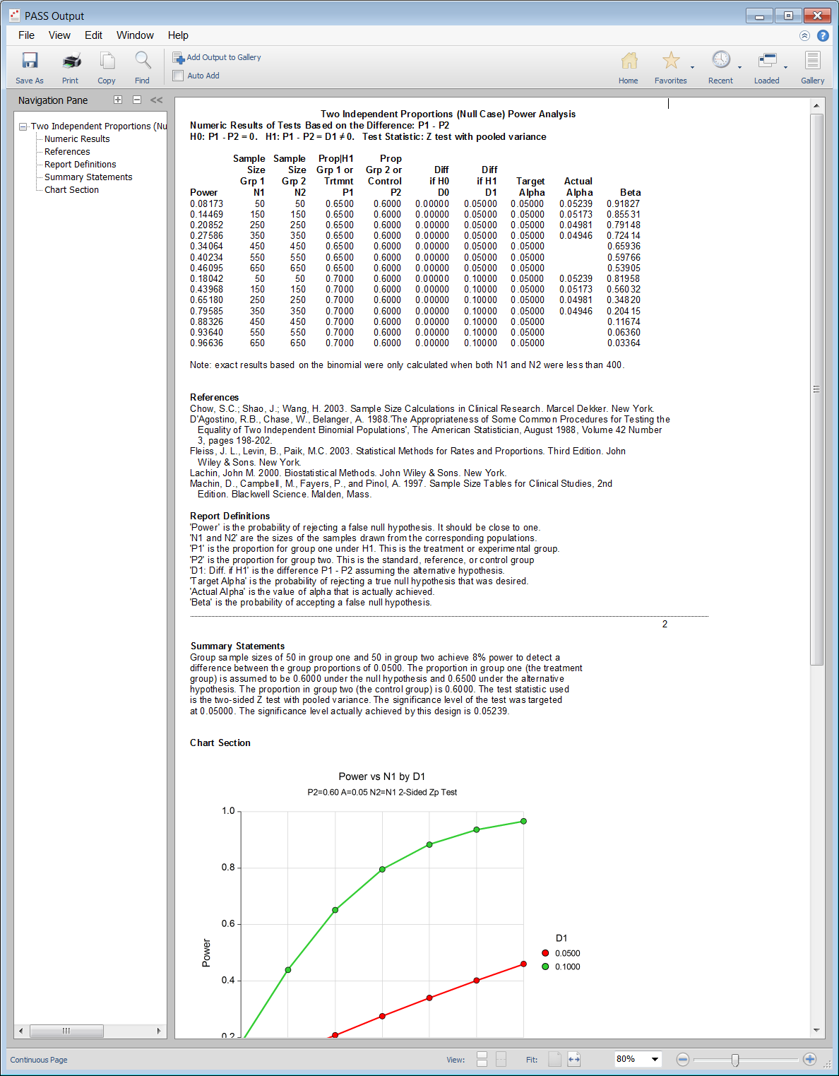
In a typical two proportion test procedure where the goal is to estimate the sample size, the user enters power, alpha, and the desired population proportions. The procedure is run and the output shows a summary of the entries as well as the sample size estimate. A summary statement is given, as well as references to the articles from which the formulas for the result were obtained.
For many of the parameters (e.g., power, alpha, sample size, proportions, etc.), multiple values may be entered in a single run. When this is done, estimates are made for every combination of entered values. A numeric summary of these is results is produced as well as easy-to-read sample size or power curve graphs.
Technical Details
This page provides a brief description of the tools that are available in PASS for power and sample size analysis of two proportions. If you would like to examine the formulas and technical details relating to a specific PASS procedure, we recommend you
download and install the free trial of the software, open the desired proportions procedure, and click on the help button in the top right corner to view the complete documentation of the procedure. There you will find summaries, formulas, references, discussions, technical details, examples, and validation against published articles for the procedure.
An Example Setup and Output
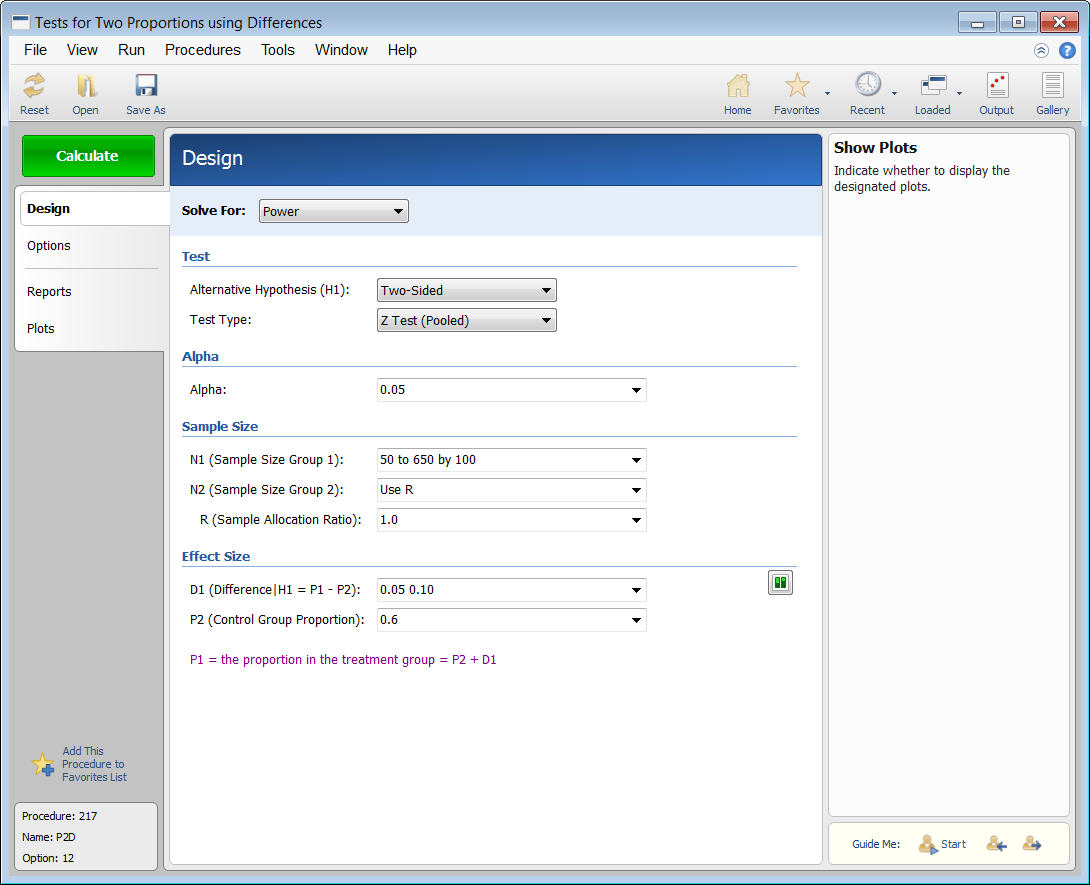
When the PASS software is first opened, the user is presented with the PASS Home window. From this window the desired procedure is selected from the menus, the category tree on the left, or with a procedure search. The procedure opens and the desired entries are made. When you click the Calculate button the results are produced. You can easily navigate to any part of the output with the navigation pane on the left.
PASS Home Window

Procedure Window for Tests for One Proportion

PASS Output Window

Sample Size for Inequality Tests for Two Independent Proportions
This procedure computes power and sample size for hypothesis tests of the difference, ratio, or odds ratio of two independent proportions. The test statistics analyzed by this procedure assume that the difference between the two proportions is zero or their ratio is one under the null hypothesis. This procedure computes and compares the power achieved by each of several test statistics that have been proposed. The power calculations assume that random samples are drawn from two separate populations.
The available test statistics in these procedures include:
- Fisher’s Exact Test
- Z-Test (Pooled)
- Z-Test (Unpooled)
- Z-Test with Continuity Correction (Pooled)
- Z-Test with Continuity Correction (Unpooled)
- Conditional Mantel Haenszel
- Likelihood Ratio Test
Sample Size for Tests for Two Proportions using Effect Size
This procedure provides sample size and power calculations for one- or two-sided hypothesis tests of the difference between two independent proportions using the effect size. The details of procedure are given in Cohen (1988).
Sample Size for Confidence Intervals for Two Proportions
This routine calculates the group sample sizes necessary to achieve a specified interval width of the difference, ratio, or odds ratio of two independent proportions.
Calculations may be made for several different confidence interval formulas for differences, ratios, and odds ratios.
Formulas for the Difference
- Farrington and Manning’s Score
- Miettinen and Nurminen’s Score
- Gart and Nam’s Score
- Wilson’s Score as Modified by Newcombe
- Wilson’s Score as Modified by Newcombe with Continuity Correction
- Yate’s Chi-Square with Continuity Correction
- Pearson’s Chi-Square
Formulas for the Ratio
- Farrington and Manning’s Score
- Miettinen and Nurminen’s Score
- Gart and Nam’s Score
- Logarithm (Katz)
- Logarithm (Walters)
- Iterated Method of Fleiss
Formulas for the Odds Ratio
- Conditional Exact
- Farrington and Manning’s Score
- Miettinen and Nurminen’s Score
- Iterated Method of Fleiss
- Logarithm
- Mantel-Haenszel
- Simple
- Simple + 1/2
Sample Size for Non-Inferiority Tests for Two Proportions
These procedures provide power analysis and sample size calculation for non-inferiority tests in two-sample designs in which the outcome is binary. There are four non-inferiority procedures for two proportions. These procedures are identical except for the type of parameterization. The parameterization can be in terms of proportions, differences in proportions, ratios of proportions, and odds ratios. Users may choose from among several popular test statistics commonly used for running the hypothesis test.
The available test statistics in these procedures include:
- Z-Test (Pooled)
- Z-Test (Unpooled)
- Z-Test with Continuity Correction (Pooled)
- Z-Test with Continuity Correction (Unpooled)
- Likelihood Score (Farrington and Manning)
- Likelihood Score (Miettinen and Nurminen)
- Likelihood Score (Gart and Nam)
Sample Size for Equivalence Tests for Two Proportions
These procedures provide power analysis and sample size calculation for equivalence tests in two-sample designs in which the outcome is binary. There are four equivalence procedures for two proportions. These procedures are identical except for the type of parameterization. The parameterization can be in terms of proportions, differences in proportions, ratios of proportions, and odds ratios. Users may choose from among several popular test statistics commonly used for running the hypothesis test.
The available test statistics in these procedures include:
- Z-Test (Pooled)
- Z-Test (Unpooled)
- Z-Test with Continuity Correction (Pooled)
- Z-Test with Continuity Correction (Unpooled)
- Likelihood Score (Farrington and Manning)
- Likelihood Score (Miettinen and Nurminen)
- Likelihood Score (Gart and Nam)
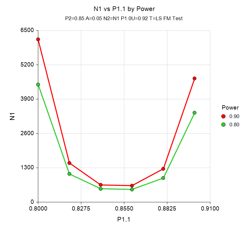
Equivalence Test Sample Size Curve

Sample Size for Superiority by a Margin Tests for Two Proportions
These procedures provide power analysis and sample size calculation for superiority by a margin tests in two-sample designs in which the outcome is binary. There are four superiority procedures for two proportions. These procedures are identical except for the type of parameterization. The parameterization can be in terms of proportions, differences in proportions, ratios of proportions, and odds ratios. Users may choose from among several popular test statistics commonly used for running the hypothesis test.
The available test statistics in these procedures include:
- Z-Test (Pooled)
- Z-Test (Unpooled)
- Z-Test with Continuity Correction (Pooled)
- Z-Test with Continuity Correction (Unpooled)
- Likelihood Score (Farrington and Manning)
- Likelihood Score (Miettinen and Nurminen)
- Likelihood Score (Gart and Nam)
Sample Size for Tests for Two Proportions in a Repeated Measures Design
There are two procedures for two proportions in a repeated measures design. These procedures are identical except for the type of parameterization. The parameterization can be in terms of proportions or odds ratios.
These procedures calculate the power for testing the time-averaged difference (TAD) between two proportions in a repeated measures design. A repeated measures design is one in which subjects are observed repeatedly over time. Measurements may be taken at pre-determined intervals (e.g. weekly or at specified time points following the administration of a particular treatment), or at random times with variable intervals between repeated measurements.
This type of time-averaged difference analysis is often used when the outcome to be measured varies with time. For example, suppose that you want to compare two treatment groups based on a certain binary response variable such as the presence (or absence) of a disease. The disease status may change over time, depending on various factors unrelated to the treatment. The precision of the experiment is increased by taking multiple measurements from each individual and comparing the time-averaged difference in proportions between the two groups. Care must be taken in the analysis because of the correlation that is introduced when several measurements are taken from the same individual. The covariance structure may take on several forms depending on the nature of the experiment and the subjects involved. This procedure allows you to calculate sample sizes and power using four different covariance patterns: Compound Symmetry, AR(1), Banded(1), and Simple.
These procedures can be used to calculate sample size and power for tests of pairwise contrasts in a mixed models analysis of repeated measures data. Mixed models analysis of repeated measures data is also employed to provide more flexibility in covariance specification and a greater degree of robustness in the presence of missing data, provided that the data can be assumed to be missing at random.
Sample Size for Group-Sequential Tests for Two Proportions
There are a number of group sequential procedures in PASS for the comparison of two proportions. One analytic procedure is available as well as simulation procedures for each of the following test types:
- Group-Sequential Tests for the Difference of Two Proportions
- Group-Sequential Non-Inferiority Tests for the Difference of Two Proportions
- Group-Sequential Superiority by a Margin Tests for Two Proportions
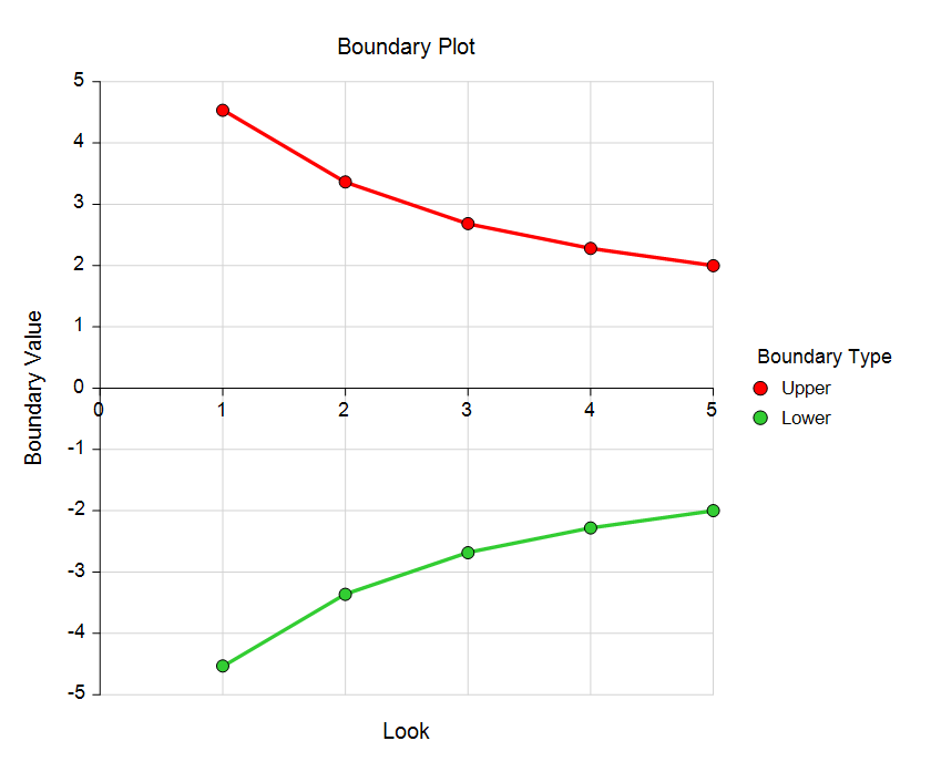
A variety of spending function options are available in these procedures, including Hwang-Shi-DeCani, O’Brien-Fleming, and Pocock types. Either the T-test or the Mann-Whitney-Wilcoxon test may be examined. For one-sided tests, significance and futility boundaries can be produced. The spacing of the looks can be equal or custom specified. The distributions of each of the groups under the null and alternative hypotheses can be specified directly using over ten distributions including normal, exponential, Gamma, Uniform, Beta, and Cauchy. Boundaries can also be input directly to verify alpha- and/or beta-spending properties. Futility boundaries can be binding or non-binding.
Group-Sequential Test Boundary Plot with 5 Looks

Sample Size for Group-Sequential Tests for Two Proportions (Simulation)
This procedure can be used to determine power, sample size and/or boundaries for group-sequential tests comparing the proportions of two groups. The available Z-tests are the common Wald Z-test using the unpooled variance estimate, with or without the continuity correction. For one- and two-sided tests, efficacy and/or futility boundaries can be generated. The spacing of the stages can be equal or custom specified. Individual stages may also be skipped. Boundaries can be computed based on popular alpha- and beta-spending functions (O’Brien-Fleming Analog, Pocock Analog, Hwang-Shih-DeCani Gamma family, linear) or custom spending functions, or boundaries may be input directly, if desired. Futility boundaries can be binding or non-binding. Corresponding P-Value boundaries are given for each boundary statistic. Alpha and/or beta spent at each stage is reported. Plots of boundaries are also produced.
This procedure is used as the planning tool for determining sample size and initial boundaries. Stage data, as it is obtained, can be evaluated using the companion procedure Group-Sequential Analysis for Two Proportions. The companion procedure also gives the option for sample-size re-estimation and updated boundaries for current-stage information. In that procedure, simulation can be used to evaluate boundary-crossing probabilities given the current stage results.
Sample Size for Group-Sequential Non-Inferiority Tests for Two Proportions (Simulation)
This procedure can be used to determine power, sample size and/or boundaries for group-sequential tests comparing the proportions of two groups. The available Z-tests are the common Wald Z-test using the unpooled variance estimate, with or without the continuity correction, and with a non-inferiority margin.
Stage data, as it is obtained, can be evaluated using the companion procedure Group-Sequential Non-Inferiority Analysis for Two Proportions.
Sample Size for Group-Sequential Superiority by a Margin Tests for Two Proportions (Simulation)
This procedure can be used to determine power, sample size and/or boundaries for group-sequential tests comparing the proportions of two groups. The available Z-tests are the common Wald Z-test using the unpooled variance estimate, with or without the continuity correction, and with a superiority margin.
Stage data, as it is obtained, can be evaluated using the companion procedure Group-Sequential Superiority by a Margin Analysis for Two Proportions.
Sample Size for Conditional Power of Two Proportions Tests
This procedure computes conditional and predicted power for the case when a test is used to test whether the event probabilities of two populations are different.
In sequential designs, one or more intermediate analyses of the emerging data are conducted to evaluate whether the experiment should be continued. This may be done to conserve resources or to allow a data monitoring board to evaluate safety and efficacy when subjects are entered in a staggered fashion over a long period of time. Conditional power (a frequentist concept) is the probability that the final result will be significant, given the data obtained up to the time of the interim look. Predictive power (a Bayesian concept) is the result of averaging the conditional power over the posterior distribution of effect size. Both of these methods fall under the heading of stochastic curtailment techniques.
Conditional power procedures are also available in PASS for the case of Non-Inferiority and Superiority by a Margin.
Sample Size for Tests for Two Proportions in a Stratified Design (Cochran/Mantel-Haenszel Test)
In a stratified design, the subjects are selected from two or more strata which are formed from important covariates such as gender, income level, or marital status. The number of subjects in each of the two groups in each strata is set (fixed) by the design. A separate 2-by-2 table is formed for each stratum. Although response rates may vary among strata, hypotheses about the overall odds ratio can be tested the Cochran-Mantel-Haenszel test. This procedure allows you to determine power and sample size for such a study.
Sample Size for Tests for Two Proportions in a Cluster-Randomized Design
A number of procedures are available in PASS for the comparing two proportions in a cluster-randomized design. Below is a list of procedure categories of this type:
- Inequality Tests for Two Proportions in a Cluster-Randomized Design
- Non-Inferiority Tests for Two Proportions in a Cluster-Randomized Design
- Equivalence Tests for Two Proportions in a Cluster-Randomized Design
- Superiority by a Margin Tests for Two Proportions in a Cluster-Randomized Design
A cluster (group) randomized design is one in which whole units, or clusters, of subjects are randomized to the groups rather than the individual subjects in those clusters. However, the conclusions of the study concern individual subjects rather than the clusters. Examples of clusters are families, school classes, neighborhoods, and hospital wards.
Cluster-randomized designs are often adopted when there is a high risk of contamination if cluster members were randomized individually. For example, it may be difficult for an instructor to use two methods of teaching individuals in the same class. The price of randomizing by clusters is a loss of efficiency--the number of subjects needed to obtain a certain level of precision in a cluster-randomized trial is usually much larger than the number needed when the subjects are randomized individually. Hence, the basic two-sample methods of sample size estimation cannot be used.
Sample Size for Two Proportions in a Stepped-Wedge Cluster-Randomized Design
A stepped-wedge cluster-randomized design is similar to a cross-over design in that each cluster receives both the treatment and control over time. In a stepped-wedge design, however, the clusters switch or cross-over in one direction only (usually from the control group to the treatment group). Once a cluster is randomized to the treatment group, it continues to receive the treatment for the duration of the study. In a typical stepped-wedge design the all clusters are assigned to the control group at the first time point and then individual clusters are progressively randomized to the treatment group over time. The stepped-wedge design is particularly useful for cases where it is logistically impractical to apply a particular treatment to half of the clusters at the same time.
This procedure computes power and sample size for tests for the difference between two proportions in cross-sectional stepped-wedge cluster-randomized designs. In cross-sectional designs, different subjects are measured within each cluster at each point in time. No one subject is measured more than once. (This is not to be confused with cohort studies (i.e. repeated measures) where individuals are measured at each point in time. The methods in this procedure should not be used for cohort or repeated measures designs.)
Sample Size for Tests for Two Proportions in a Split-Mouth Design
This procedure assumes that binary data will be obtained from a study that uses a split-mouth design. The GEE method is used to analyze the repeated measures model that is assumed. The sample size formula is derived in Zhu, Zhang, and Ahn (2017).
A split-mouth design is used in dental trials in which treatments are randomized over segments of the mouth within each subject. In this design, the mouth is divided into two or more segments or regions. For example, the segments might be top and bottom, left and right, or a combination of both. Within each segment, specific sites (e.g. teeth) are identified. The same treatment is applied to all sites within a segment.
The split-mouth design, also called the split-cluster design, is occasionally used in other areas such as dermatology and animal studies. Although the design may be used in other experiments, the terminology of the split-mouth design will be used in this procedure.
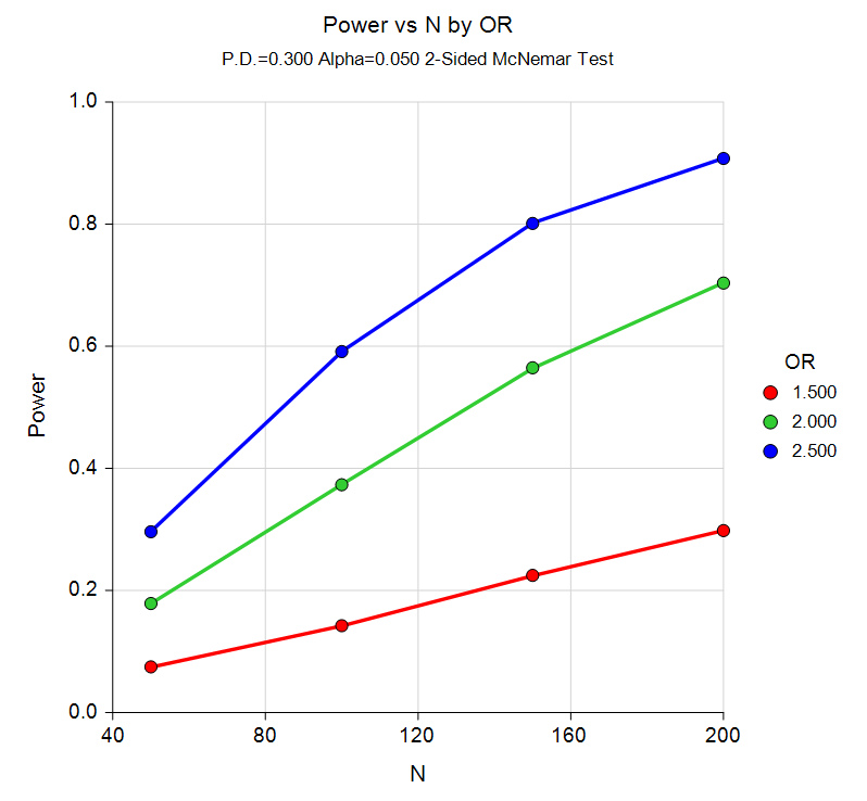
Sample Size for Tests for Two Correlated Proportions (McNemar Test)
This procedure permits sample size and power analysis for studies where the analysis is to done based on the McNemar test.
McNemar Test Power Curve

Sample Size for Tests for Two Correlated Proportions in a Matched Case-Control Design
A 2-by-M case-control study investigates a risk factor relevant to the development of a disease. A population of case patients with a disease and control patients without the disease is considered. Some of these patients have had exposure to a risk factor of interest. A random sample of N case patients is selected. Patients are stratified by the levels of a confounding variable (such as age, gender, etc.). For each selected case patient, a random sample of M matched control patients is drawn from the same strata (group). An estimate of the odds ratio, OR, of developing the disease in exposed and unexposed patients who have equal values of the confounding variable is desired. This odds ratio is assumed to be constant across all levels of the confounding variables.
This procedure permits the user to solve for power, or for the number of cases, or for the number of controls per case.
Sample Size for Tests for the Matched-Pair Difference of Two Proportions in a Cluster-Randomized Design
Cluster-randomized designs are those in which whole clusters of subjects (classes, hospitals, communities, etc.) are sampled, rather than individual subjects. This sample size and power procedure is used for the case where the subject responses are binary (proportion outcome). To reduce the variation (and thus increase power), clusters are matched, with one cluster of each pair assigned to the control group, and the other assigned the treatment group. This procedure gives the number of pairs needed for the desired power requirement.
Sample Size for GEE Tests for Two Correlated Proportions with Dropout
This procedure provides power analysis and sample size calculation for studies that use a paired design that yield two binary outcomes, one of which may be incomplete. That is, in some pairs, the second observation is missing. The data analysis will use a mixed logistic regression model that is solved with GEE.
With complete data, the standard analysis is McNemar’s Test (see McNemar (1947)), and PASS includes several procedures that analyze that test statistic. McNemar’s Test requires that observations with one or two missing observations must be discarded. Zhang, Cao, and Ahn (2014) present a closed-form sample size formula for the case when some data pairs include missing values in the second observation. This is often referred to as dropout.
Another method, also available for sample size calculation in PASS, deals with the important case in which all missing values occur in the second observation. We refer to this as dropout. We refer to that procedure for further details.
Sample Size for Tests for Two Correlated Proportions with Incomplete Observations
This procedure provides power analysis and sample size calculation for studies that use a paired design that yield two binary outcomes that may be incomplete. That is, in some pairs, either the first or the second observation is missing, but not both.
Without incomplete data, the standard analysis is McNemar’s Test (see McNemar (1947)), and PASS includes several procedures that analyze this test. This test requires that observations with at least one missing observation must be discarded. Zhang, Cao, and Ahn (2017) present sample size formulas for two extensions of McNemar’s Test that use the information provided by pairs that are only partially observed. The first method uses a test that is the result of Thompson (1995), Ekbohm (1982), and Choi and Stablein (1982) the requires the estimation of the two marginal probabilities from the complete and the partial data. The difference of these two estimates is then used for the test.
The second method, proposed by Zhang, Cao, and Ahn (2017), uses the differences between observational pairs directly. This allows this method to be more efficient in most (but not all) situations.
Another method, also available for sample size calculation in PASS, deals with the important case in which all missing values occur in the second observation. We refer to this as dropout. We refer to that procedure for further details.

