Getting Started

Description:

Hello and welcome to this quick start tour of PASS. In this video, we’ll guide you through a simple sample size calculation using the Two-Sample T-test procedure to highlight some of the important features and capabilities of the software.

When you start PASS, the first window that appears is called the PASS Home window. This window is primarily used to find and load power and sample size calculation procedures. You can find any procedure by entering key words in the search bar… or you can locate a procedure using the category tree. As you select each topic in the tree, a list of associated procedures is displayed. You can shorten the list by expanding the tree and selecting subcategories.

To find the Two-Sample T-test procedure, we expand Means, Two Independent Means, and then click on T-Test. Now we’re presented with a short list of available procedures associated with this topic. Click on the view buttons to change how this list is displayed. For this demonstration we’ll calculate sample size for the Equal Variance T-Test. The choices indicate that we can specify the effect size using differences or means. Let’s load the procedure that uses differences.

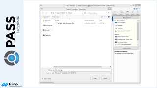
The window that now appears is called the Procedure window. This window contains all of the calculation input parameters and options organized on tabs. The important design parameters that directly affect power and sample size calculations are contained on the upper-most tabs, located above the horizontal line. You should consider every option on each of these tabs before running your sample size calculation. The actual options on these tabs vary from procedure to procedure, but the layout will be similar to what you see here.

Additional report and plot customization options are provided on the tabs located below the horizontal line. These options do not affect calculations and do not always need to be considered. The options on tabs below the line are about the same in every procedure. The Help Pane provides several resources to help you use PASS effectively. As you mouse over each option, the Option Info section provides in-depth information.

If you’d like more help, expand the Help Center. The Help Center contains links to online training videos and the procedure documentation. Each procedure in PASS is fully-documented, with technical details, examples, and validation! If you don’t want to see the options in the Help Center, you can collapse it.

Let’s now specify the input parameters for a simple sample size calculation according to an example study design. Each procedure has different input parameters, but as we fill in the options for the T-test, you’ll become familiar with how it’s done generally. First, choose the parameter to solve for based on the other input parameters. In this example, we’ll solve for sample size. Next, leave the hypothesis test direction as two-sided, the default value.

Enter 0.8 for power to calculate the sample size required to achieve 80% power. Let’s leave alpha at 0.05 and assume equal group sample size allocation; both are the defaults. For delta, the difference in means to detect, enter 5, and for sigma, the standard deviation of both groups, enter 15.

That’s it! We’ve entered all the information needed to perform this sample size calculation. Click the green Calculate button to get the results. The report is displayed in the output window. The Numeric Results Section reports that the sample size required to achieve 80% power for this combination of design parameters is 143 per group, for a total of 286.

The report also includes optional literature references, report definitions and a summary statement about the results in the table. There was no plot generated in this case because it would contain only one point. By default, plots are only generated when there are enough data points to produce a meaningful graph.

Suppose now that we want to investigate the sample size for a variety of combinations of the input parameters. To do this, we’ll go back to the t-test procedure window and enter multiple values for some of the parameters. For Power we’ll enter 0.8 and 0.9 to calculate the required sample sizes to achieve 80% and 90% power. For delta, let’s enter the values 5 to 10 by 1 to investigate a range of detectable differences.

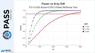
For sigma, we can enter the list 10 15 and 20 to study a range of plausible group standard deviation values. Again, click the green Calculate button to calculate the results and generate the report. This time, several sample size calculations have been made, one for each combination of the input parameters. The group sample sizes range from 17 to 337.

Since the report is lengthy, use the navigation pane to quickly jump to various sections in the report. As you can see, several sample size charts were generated this time because 3 of the input parameters were assigned multiple values. These charts provide a graphical representation of the numeric results. As expected, the required sample sizes increase with the standard deviation and the desired power. The impact is much larger for smaller group differences than it is for larger differences.

Suppose now that we want to make a few changes to the appearance of the report and the plots. To do this, we’ll go back to the Two-Sample T-Test procedure window, make the changes, and re-run the procedure. On the Reports tab, let’s force the report to show more decimals for Power by changing the number of decimal places to 7. Let’s also remove the non-essential sections from the report.

On the Plots tab, let’s change the way sample size is plotted so that Total Sample Size is displayed instead of the group sample sizes. Let’s also remove some of the 3D plots from the report. The charts currently have difference on the X-axis. Let’s change the X-Axis Parameter for the 2D plot to standard deviation. Now, click on the 2D Plot Format button and change the legend so that it appears inside the plot. Notice that the sample plot displayed on the window is updated each time we make a change.

Let’s also check the option so that we can edit the 3D plot while the procedure is running. Now we’ll use the Plot Text tab to change some of the title and label abbreviations. Change N to “Sample Size”, Delta to “Difference”, and Sigma to “Standard Deviation”. We’ve made quite a few custom changes to the report. The settings we have entered are automatically saved when the procedure is closed and will be reloaded with the procedure when it is opened again.

Since the procedure is set up just right, let’s go one step further and save these settings to a file, which will allow us to use these exact settings at any time, even after Resetting all options to their defaults. Since we are going to use this procedure in the future, let’s also add it to the favorites list by clicking on the Add to Favorites button. This will allow us to easily find it at any time. Your favorite and recent procedures can be accessed from the toolbar on all of the major windows in PASS.

Now, click the green “Calculate” button to get the results. The calculations will stop before the report is generated to allow you to edit the 3D plot. Let’s first change the colors on the plot. To change the plot’s 3D orientation, left-click on the plot preview and drag your mouse. Click OK to save the settings and view the report.

Notice that the values for Power are now displayed with 7 decimal places. The plots have also changed according to our specifications, with total sample size now being displayed on the y-axis and standard deviation on the X-axis of the 2 dimensional plots. Double-click any graph to enlarge it. All plots can easily be saved to any one of several file formats.

This report looks just right, so let’s save it to the gallery by clicking the Add Output to Gallery button. This will allow us to compare this report to other calculations later on in this session. The output window is cleared each time a new report is generated, but the gallery is not. You can easily switch between the gallery and the output using the navigation buttons in the toolbar. We can also save the entire report, or easily copy and paste individual sections into a document or presentation!