Design of Experiments in NCSS
NCSS includes several tools for designing experiments. Use the links below to jump to the design of experiments topic you would like to examine. To see how these tools can benefit you, we recommend you download and install the free trial of NCSS. For sample size and power analysis calculation tools, take a look at NCSS’s companion software PASS (Power Analysis and Sample Size). Jump to:- Introduction
- Technical Details
- Randomization Lists
- Balanced Incomplete Block Designs
- Fractional Factorial Designs
- Latin Square Designs
- Response Surface Designs
- Screening Designs
- Taguchi Designs
- Two-Level Designs
- Design Generator
- D-Optimal Designs
Introduction
Experimental design is the planning of an efficient, reliable, and accurate technical study. The range of application of experimental design principles is as broad as science and industry. One person may be planning a long-term agricultural experiment, while another may have eight hours to rectify a production problem. How can we expect that the same methods are appropriate in all situations? Of course, we cannot. Through the years, researchers and statisticians working together have outlined the basic steps necessary to conduct an effective investigation. These steps form an experimental strategy that seems to work well in many settings. The experimental design procedures in NCSS lend you, the investigator, a hand with the planning and analysis of your investigation. Once you have determined the scope of your investigation, the design modules will provide a data collection plan that will minimize the amount of data collected and maximize the amount of conclusive information available.Technical Details
This page is designed to give a general overview of the capabilities of NCSS for experimental design. If you would like to examine the formulas and technical details relating to a specific NCSS procedure, click on the corresponding '[Documentation PDF]' link under each heading to load the complete procedure documentation. There you will find formulas, references, discussions, and examples or tutorials describing the procedure in detail.Randomization Lists
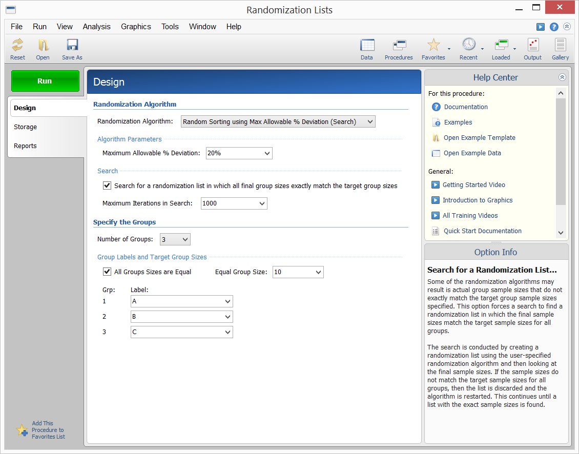
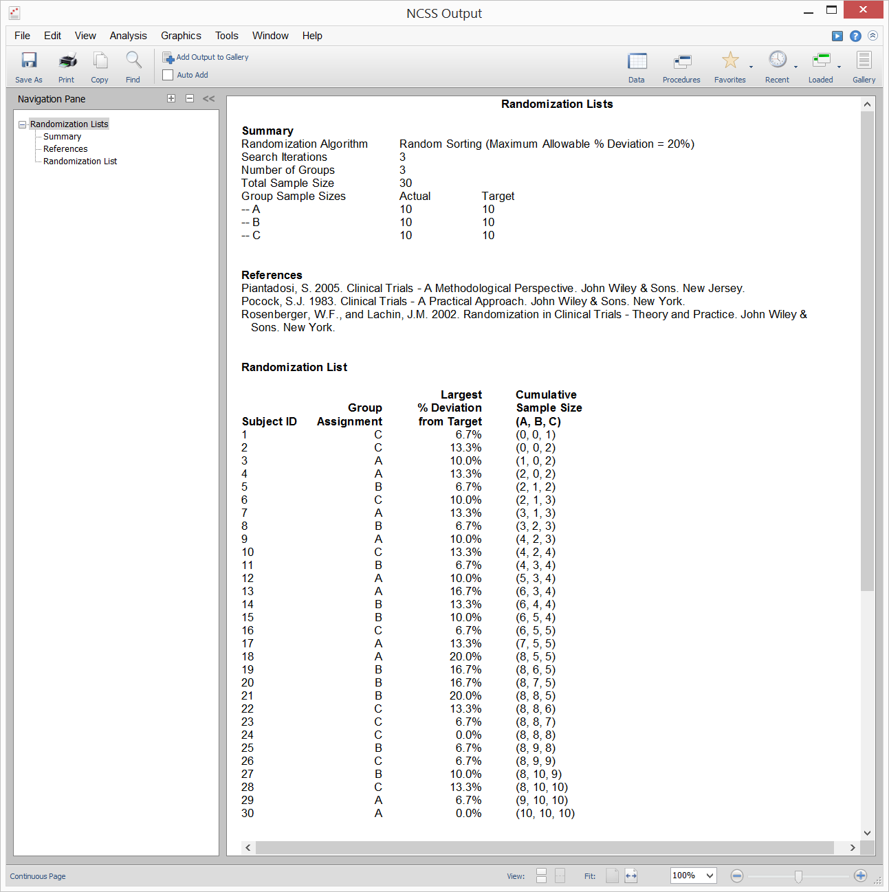
[Documentation PDF]The Randomization Lists procedure in NCSS is used to assign subjects to treatment groups. Six randomization algorithms are available. Four of the algorithms (Efron’s biased coin randomization, Smith’s randomization, Wei’s urn randomization, and random sorting using maximum allowable % deviation) are designed to generate balanced random samples throughout the course of an experiment. The other two (complete randomization and random sorting) are less complex but have higher probabilities of imbalance. Technical details for each of these algorithms (except random sorting) as well as a discussion of randomization issues in general are given in Rosenberger and Lachin (2002), Pocock (1983), and Piantadosi (2005).
Procedure Input
Sample Output
Balanced Incomplete Block Designs
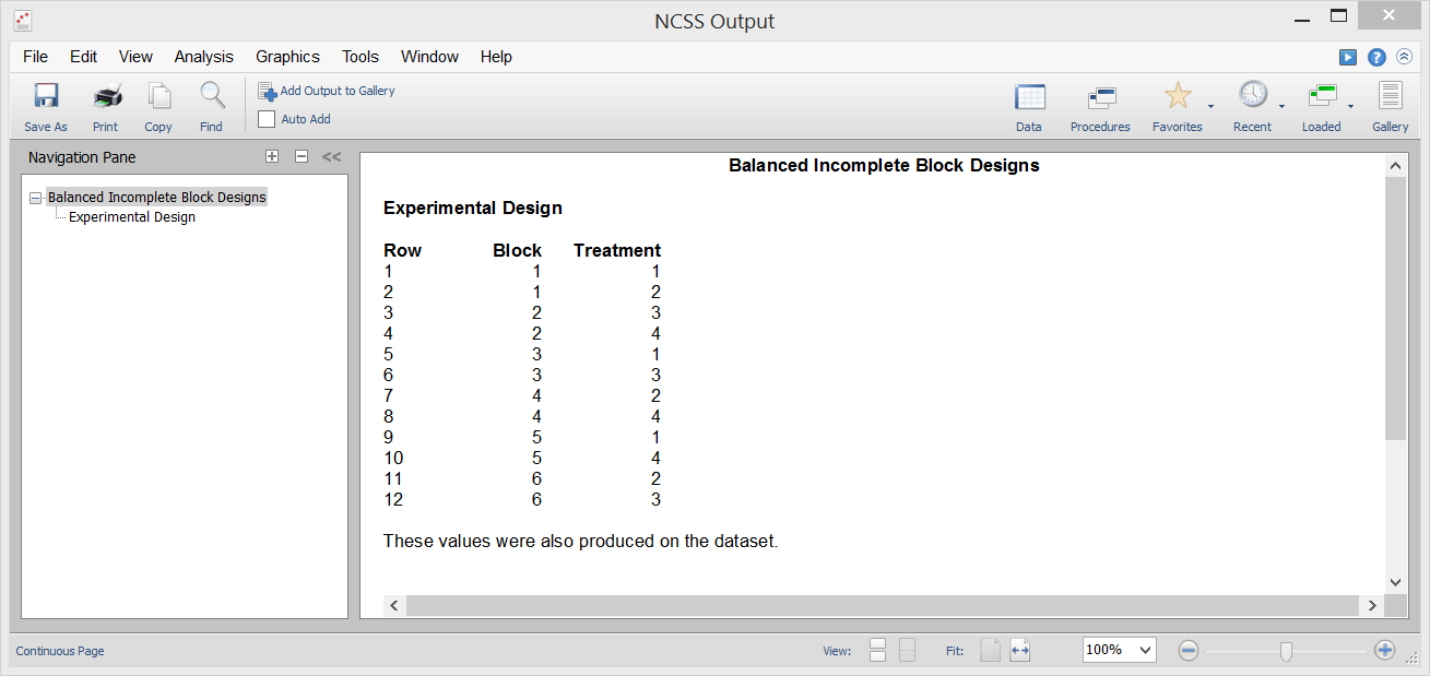
[Documentation PDF]In a balanced incomplete block design, the treatments are assigned to the blocks so that every pair of treatments occurs together in a block the same number of times. This achieves the balance that is described in the title of the procedure. The balance means that all differences between treatments are measured with equal precision. In order to make precise measurements of treatment means, uniform experimental conditions should be maintained when comparing a number of treatments. This insures that differences among the treatment means result from the application of the treatment and not from some extraneous factor. To achieve this, experimental trials are often grouped together into blocks. In such designs, conditions are kept constant within the blocks and allowed to vary between the blocks. The best known design of this type is the randomized block design. In this design, all treatments are present in each block. Occasionally, the size of convenient blocks will not accommodate all the treatments of interest. For example, suppose you wanted to test four types of automobile tires for wear. An obvious choice for a block would be an automobile. You might select ten automobiles for the study. Assuming that the tires were rotated among the four positions, this experiment would control for differences in tire wear due to the type of automobile and the terrain that each traveled. However, what would you do if you wanted to test six types of tires? You could redesign the automobile, or you could adopt a balanced incomplete block design. Following is an example of how four treatments are assigned to blocks with a natural size of three experimental units. Four blocks are required for this balanced incomplete block design.
| Block | Treatment |
| 1 | A B C |
| 2 | A B D |
| 3 | A C D |
| 4 | B C D |
Note that each treatment occurs three times in this experimental layout. Also note that each pair of treatments occurs twice. These are the basic properties of the balanced incomplete designs. Box, Hunter, and Hunter (1978) point out the following rules when using such designs.
- 1. Randomly assign the numbers to the blocks.
- 2. Randomly assign the letters to the treatments.
- 3. Randomly assign the treatments within the blocks.
- 4. Randomly group blocks as replicates. A replicate is a complete set of all treatments.
Sample Output
Fractional Factorial Designs
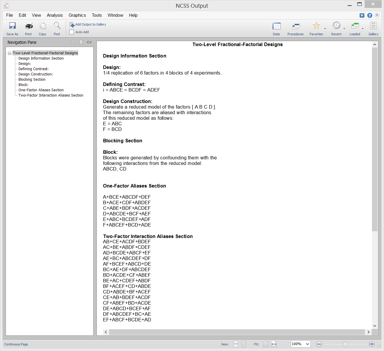
[Documentation PDF]This procedure generates two-level fractional-factorial designs of up to sixteen factors with blocking. Reports show the aliasing pattern that is used. The design rows may be output in standard or random order. When generating a design, the program first checks to see if the design is among those listed on page 410 of Box and Hunter (1978). These designs are especially good. If the requested design is not listed in the above book, the design pattern is determined using the standard procedure in which the highest-order interactions are confounded first, and so on. The procedure makes certain that main effects are not aliased with each other.
Sample Output
Latin Square Designs
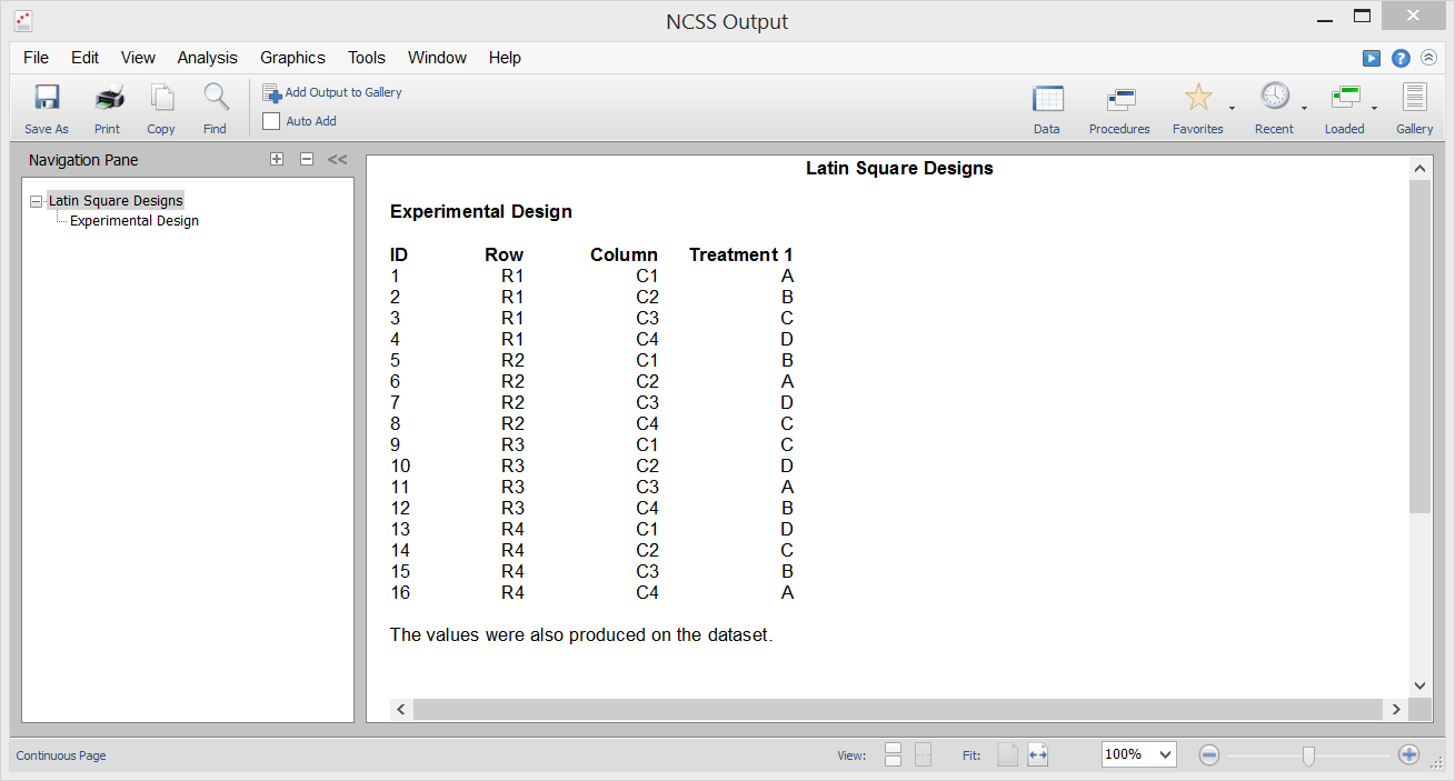
[Documentation PDF]This procedure generates Latin Square and Graeco-Latin Square designs. Designs for from three to ten treatments are available. Latin Square designs are similar to randomized block designs, except that instead of the removal of one blocking variable, these designs are carefully constructed to allow the removal of two blocking factors. They accomplish this while reducing the number of experimental units needed to conduct the experiment. Following is an example of a four treatment Latin Square. The experimental layout is as follows:
| Column 1 | Column 2 | Column 3 | Column 4 | |
| Row 1 | A | B | C | D |
| Row 2 | B | C | D | A |
| Row 3 | C | D | A | B |
| Row 4 | D | A | B | C |
In the above table, the four treatments are represented by the four letters: A, B, C, and D. The letters are arranged so that each letter occurs only once within each row and each column. Notice that a simple random design would require 4 x 4 x 4 = 64 experimental units. This Latin Square needs only 16 experimental units—a reduction of 75%! The influence of a fourth factor may also be removed from the design by introducing a second set of letters, this time lower case. This design is known as the Graeco-Latin Square.
| Column 1 | Column 2 | Column 3 | Column 4 | |
| Row 1 | Aa | Bb | Cc | Dd |
| Row 2 | Bd | Ca | Db | Ac |
| Row 3 | Cb | Dc | Ad | Ba |
| Row 4 | Dc | Ad | Ba | Cb |
Four factors at four levels each would normally require 256 experimental units, but this design only requires 16 - a reduction in experimental units of almost 94%! The Graeco-Latin Square is formed by combining to orthogonal Latin Squares. Graeco-Latin Squares are available for all numbers of treatments except six.
Sample Output
Response Surface Designs
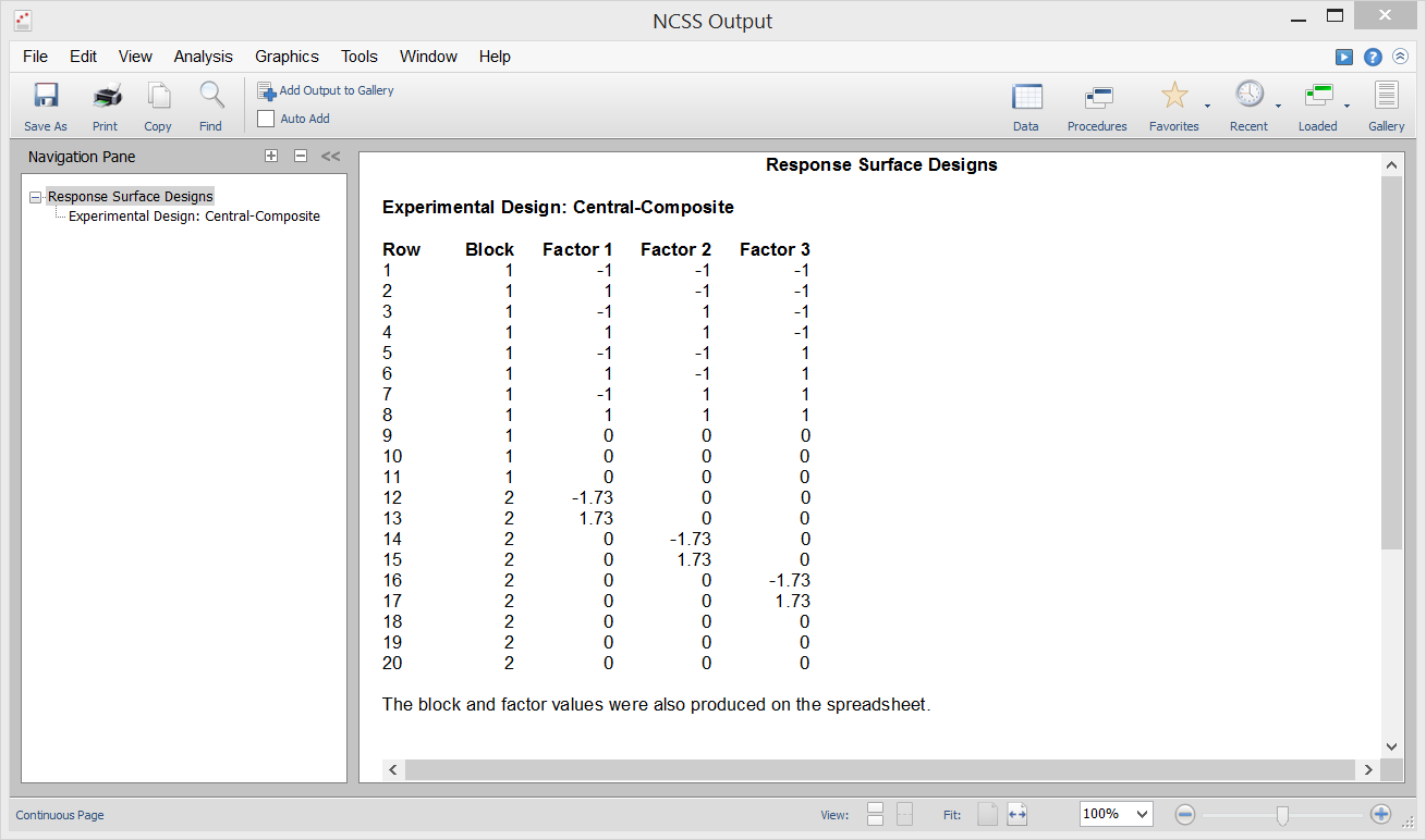
[Documentation PDF]Response-surface designs are the only designs provided that allow for more than two levels. There are two general types of response-surface designs. The central-composite designs give five levels to each factor. The Box-Behnken designs give three levels to each factor. The Central-Composite designs build upon the two-level factorial designs by adding a few center points and star points. A factor's five values are: -a, -1, 0, 1, and a. The value of a is determined by the number of factors in such a way that the resulting design is orthogonal. For example, if you are going to use either four or five factors, the value of a is 2.00. The actual values of the levels are determined from these five values as follows:
- 1. The low-level value is assigned to -1.
- 2. The high-level value is assigned to 1.
- 3. The average of these two values is assigned to 0.
- 4. The values of -a and a are used to find the minimum and the maximum values.
| Coded Level | Actual Level |
| -a | 45 |
| -1 | 50 |
| 0 | 55 |
| 1 | 60 |
| a | 65 |
The values of a depend on the number of factors in the design:
| Factors | Value of a |
| 2 | 1.41 |
| 3 | 1.73 |
| 4 | 2.00 |
| 5 | 2.00 |
| 6 | 2.24 |
The Box-Behnken designs have two differences from the central-composite designs. First, they usually use fewer runs. Second, they only use three levels while the central-composite designs use five. The actual values of the levels are determined in the same manner as the central-composite designs, except that the value of a is ignored.
Sample Output
Screening Designs
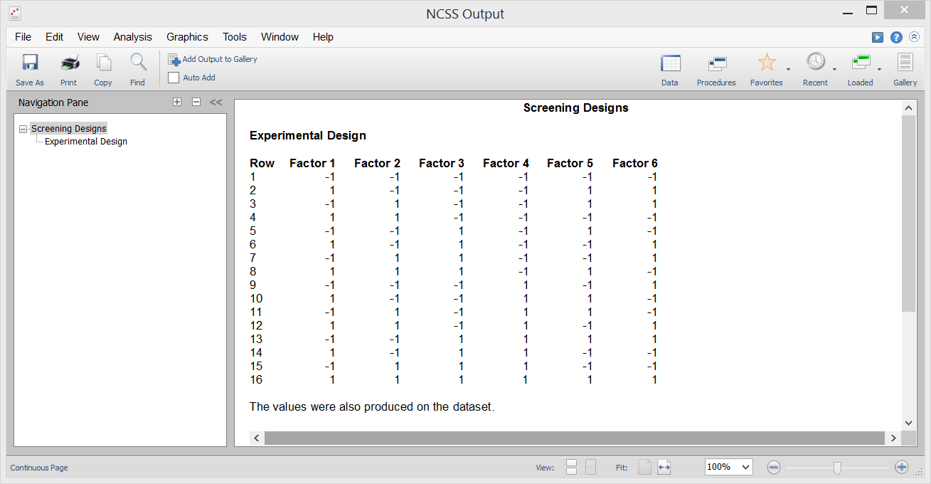
[Documentation PDF]Screening designs are used to find the important factors from a large number (up to 31) of two-level factors. When the number of runs is 4, 8, 16, or 32 (powers of 2), the design is a regular fractional replication. When the number of runs is 12, 20, 24, or 28, the design used is a Plackett-Burman design. This procedure uses the screening designs given in Lawson (1987). These designs make it possible to evaluate each main effect, although these are aliased with several interactions. When you analyze the data from these designs, it is simplest to use our Multiple Regression routine. The Analysis of Two-Level Designs program can be used to analyze designs in which the number of runs is a power of 2 (the non-Plackett Burman designs).
Sample Output
Taguchi Designs
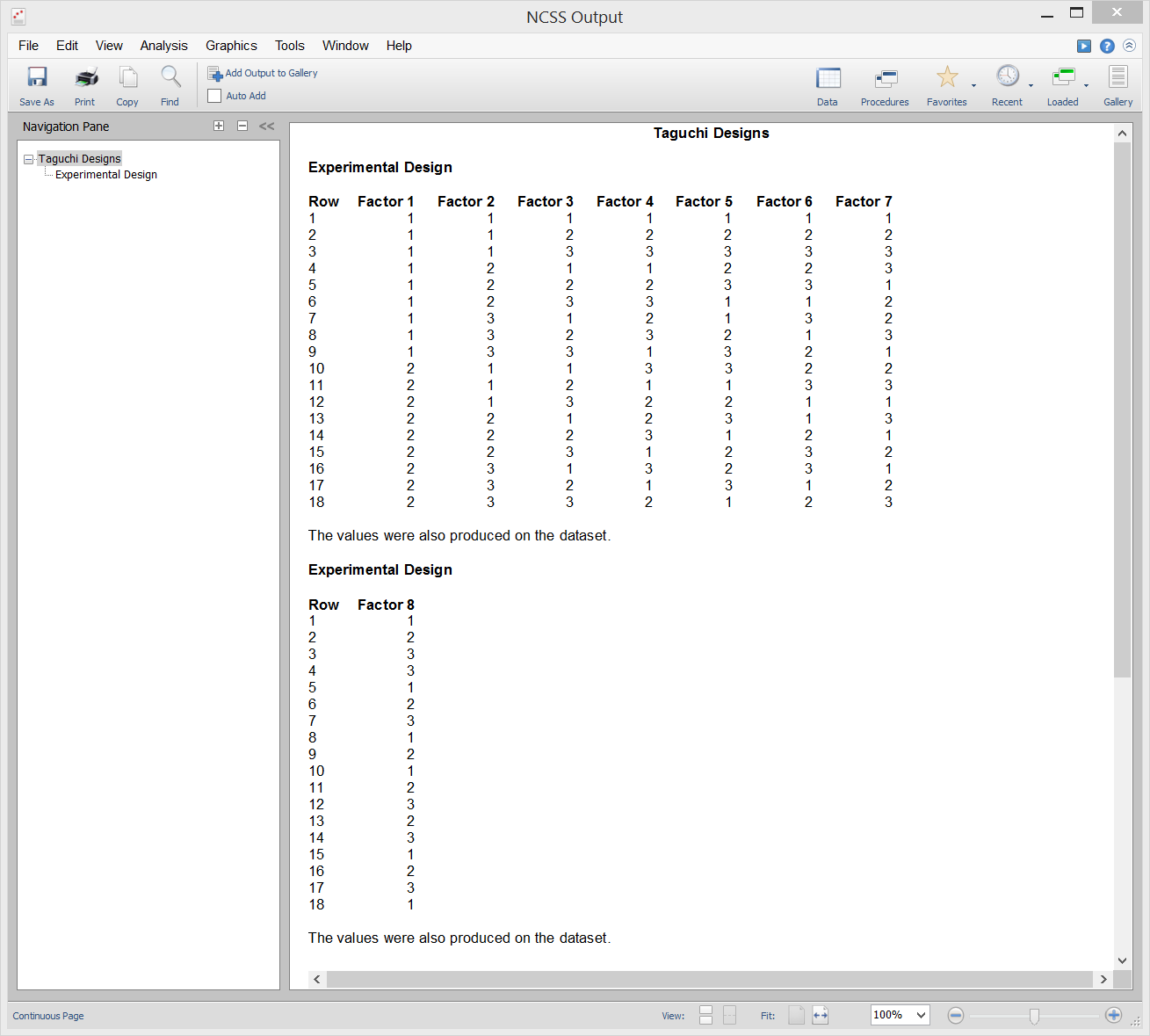
[Documentation PDF]Taguchi experimental designs, often called orthogonal arrays (OA’s), consist of a set of fractional factorial designs which ignore interaction and concentrate on main effect estimation. This program module generates the most popular set of Taguchi designs. Taguchi uses the following convention for naming the orthogonal arrays: La(b^c) where a is the number of experimental runs, b is the number of levels of each factor, and c is the number of variables. Designs can have factors with several levels, although two and three level designs are the most common. The L18 design is perhaps the most popular. When a design is generated, the levels of each factor are stored in the current dataset—replacing any data that is already there. No output reports are generated by this procedure.
Sample Output
Two-Level Designs
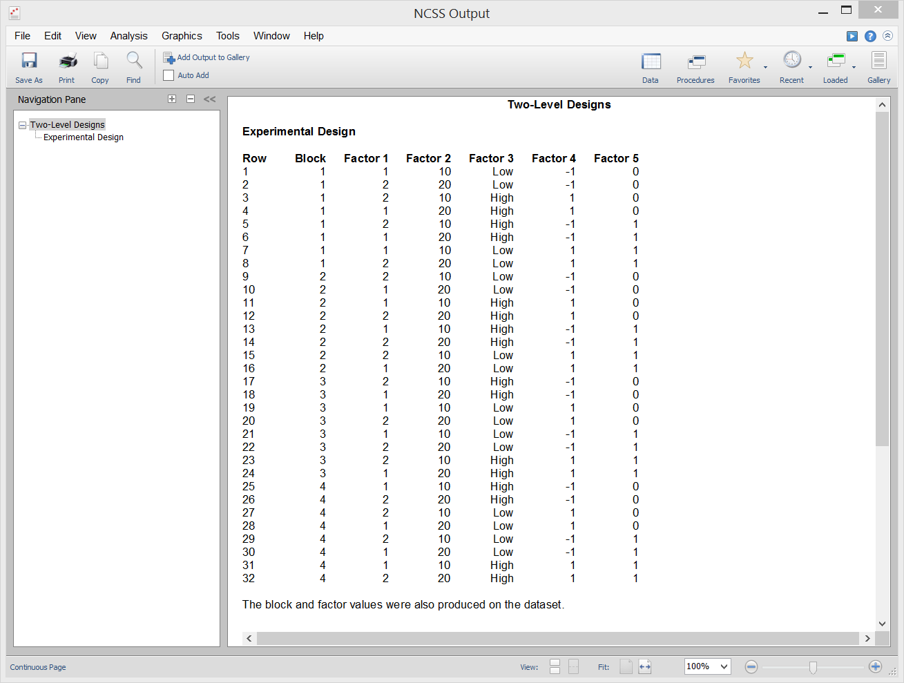
[Documentation PDF]This procedure generates a 2ᵏ factorial design for up to seven factors. It allows the design to be blocked and replicated. The design rows may be output in standard or random order. When blocking is specified, the procedure checks to see if the design is listed on page 408 of Box and Hunter (1978). If it is one of the designs specified there, the indicated confounding pattern is used. If not, the blocks are confounded using the standard procedure in which highest-order interactions are confounded first, so long as they do not cause main effects to be confounded with blocks. The blocking pattern is reported by the analysis program, so it is not reported by this program.
Sample Output
Design Generator
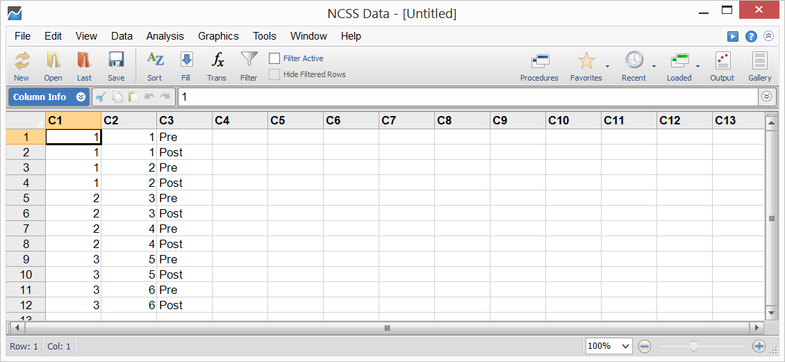
[Documentation PDF]This procedure generates factorial, repeated measures, and split-plots designs with up to ten factors. The designs are placed in the current database.
Sample Output
D-Optimal Designs
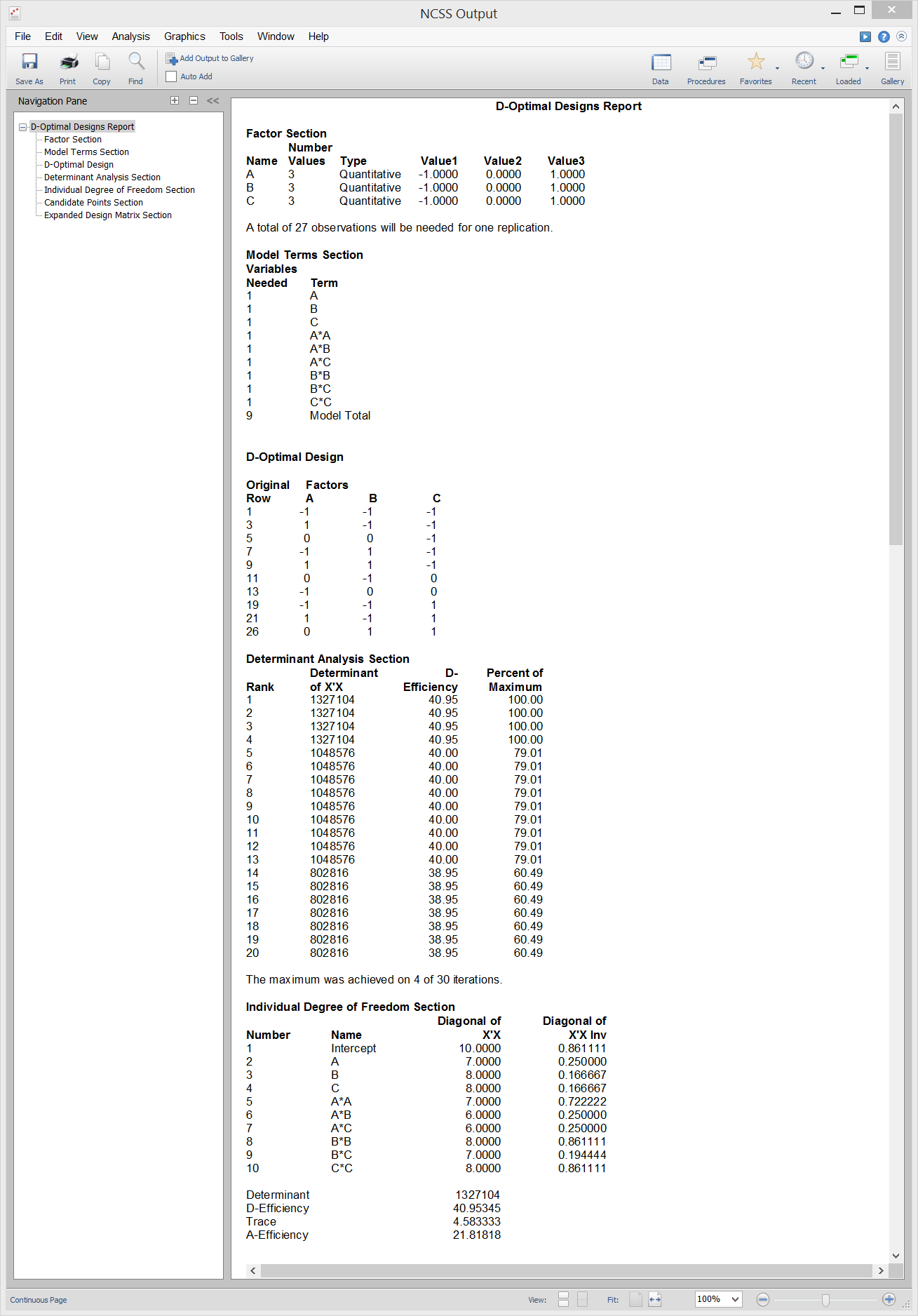
[Documentation PDF]This procedure generates D-optimal designs for multi-factor experiments with both quantitative and qualitative factors. The factors can have a mixed number of levels. Hence, you could use this procedure to design an experiment with two quantitative factors having three levels each and a qualitative factor having seven levels. D-optimal designs are constructed to minimize the generalized variance of the estimated regression coefficients. In the multiple regression setting, the matrix X is often used to represent the data matrix of independent variables. D-optimal designs minimize the overall variance of the estimated regression coefficients by maximizing the determinant of X’X. Designs that are D-optimal have been shown to be nearly optimal for several other criterion that have been proposed as well. When would you use D-optimal designs? When you have a limited budget and cannot run a completely replicated factorial design. For example, suppose you want to study the response to three factors: A with three levels, B with four levels, and C with eight levels. One complete replication of this experiment would require 3 x 4 x 8 = 96 points (we use the word ‘point’ to mean an experimental unit). Suppose you can afford only 20 points. Which 20 of the 96 possible should you use? The D-optimal design algorithm provides a reasonable choice.
Sample Output
