Sample Size for Group-Sequential Tests in PASS

PASS includes procedures for power analysis and sample size calculations for many different one-sample and two-sample group-sequential cases. The group-sequential tools in PASS are easy-to-use and validated for accuracy. For more details about group-sequential tests in PASS, we recommend you download and install the free trial of the software. For more details about group-sequential analysis and sample size re-estimation in NCSS, you can click here. Jump to:

• Introduction
• Group-Sequential Study Outline
• Technical Details
• An Example Setup and Output

Introduction

The various group-sequential sample size calculation procedures in PASS allow you to study the power and sample size for an expanding list of scenarios:

1. Tests for One Mean with Known Variance (Simulation)
2. T-Tests for One Mean (Simulation)
3. Tests for Two Means with Known Variances (Simulation)
4. T-Tests for Two Means (Simulation)
5. Tests for Two Proportions (Simulation)
6. Tests for Two Means (Simulation) Assuming Normality
7. Tests for Two Means (Simulation) General Assumptions
8. Tests for Two Means (Simulation) General Assumptions – Mann-Whitney Test
9. Non-Inferiority Tests for Two Means
10. Non-Inferiority Tests for Two Means – Mann-Whitney Test
11. Non-Inferiority Tests for Two Means with Known Variances (Simulation)
12. Superiority by a Margin Tests for Two Means with Known Variances (Simulation)
13. Non-Inferiority T-Tests for Two Means (Simulation)
14. Superiority by a Margin T-Tests for Two Means (Simulation)
15. Tests for Two Proportions
16. Tests for Two Proportions – Unequal n’s
17. Tests for Two Proportions (Simulation)
18. Tests for Two Proportions using Differences (Simulation)
19. Tests for Two Proportions using Ratios (Simulation)
20. Tests for Two Proportions using Odds Ratios (Simulation)
21. Non-Inferiority Tests for Two Proportions (Simulation)
22. Non-Inferiority Tests for Two Proportions using Differences (Simulation)
23. Non-Inferiority Tests for Two Proportions using Ratios (Simulation)
24. Non-Inferiority Tests for Two Proportions using Odds Ratios (Simulation)
25. Superiority by a Margin Tests for Two Proportions (Simulation)
26. Superiority by a Margin Tests for Two Proportions using Differences (Simulation)
27. Superiority by a Margin Tests for Two Proportions using Ratios (Simulation)
28. Superiority by a Margin Tests for Two Proportions using Odds Ratios (Simulation)
29. Non-Inferiority Tests for Two Proportions (Simulation)
30. Superiority by a Margin Tests for Two Proportions (Simulation)
31. Logrank Tests of Two Survival Curves assuming Exponential Survival
32. Logrank Tests of Two Survival Curves assuming Proportional Hazards
33. Logrank Tests (Simulation)
34. Tests for Two Hazard Rates (Simulation)
35. Non-Inferiority Tests for Two Hazard Rates (Simulation)
36. Superiority by a Margin Tests for Two Hazard Rates (Simulation)
37. Tests for One Hazard Rate (Simulation)
38. Non-Inferiority Tests for One Hazard Rate (Simulation)
39. Superiority by a Margin Tests for One Hazard Rate (Simulation)
40. Tests for Two Poisson Rates (Simulation)
41. Non-Inferiority Tests for Two Poisson Rates (Simulation)
42. Superiority by a Margin Tests for Two Poisson Rates (Simulation)
43. Tests for One Poisson Rate (Simulation)
44. Non-Inferiority Tests for One Poisson Rate (Simulation)
45. Superiority by a Margin Tests for One Poisson Rate (Simulation)

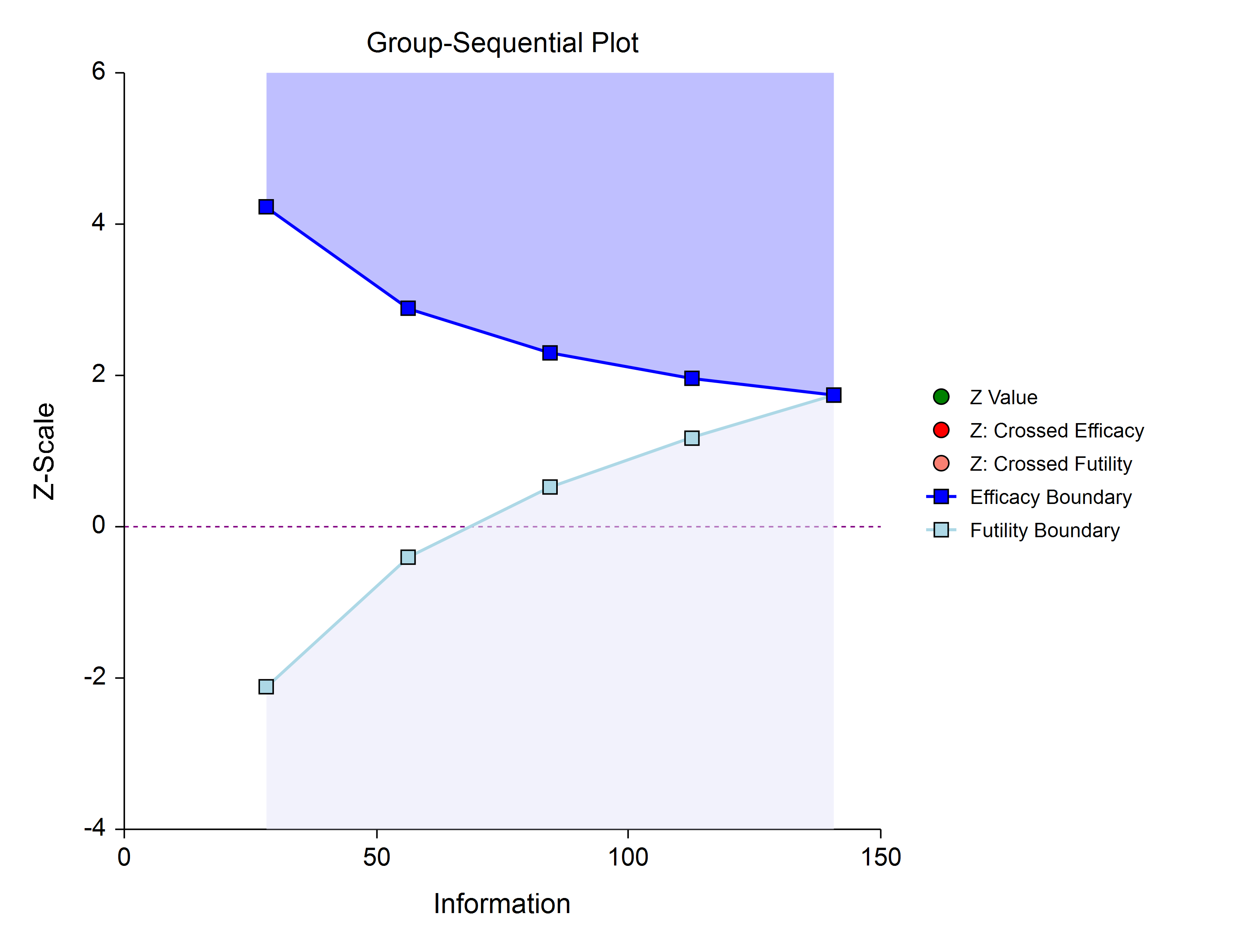
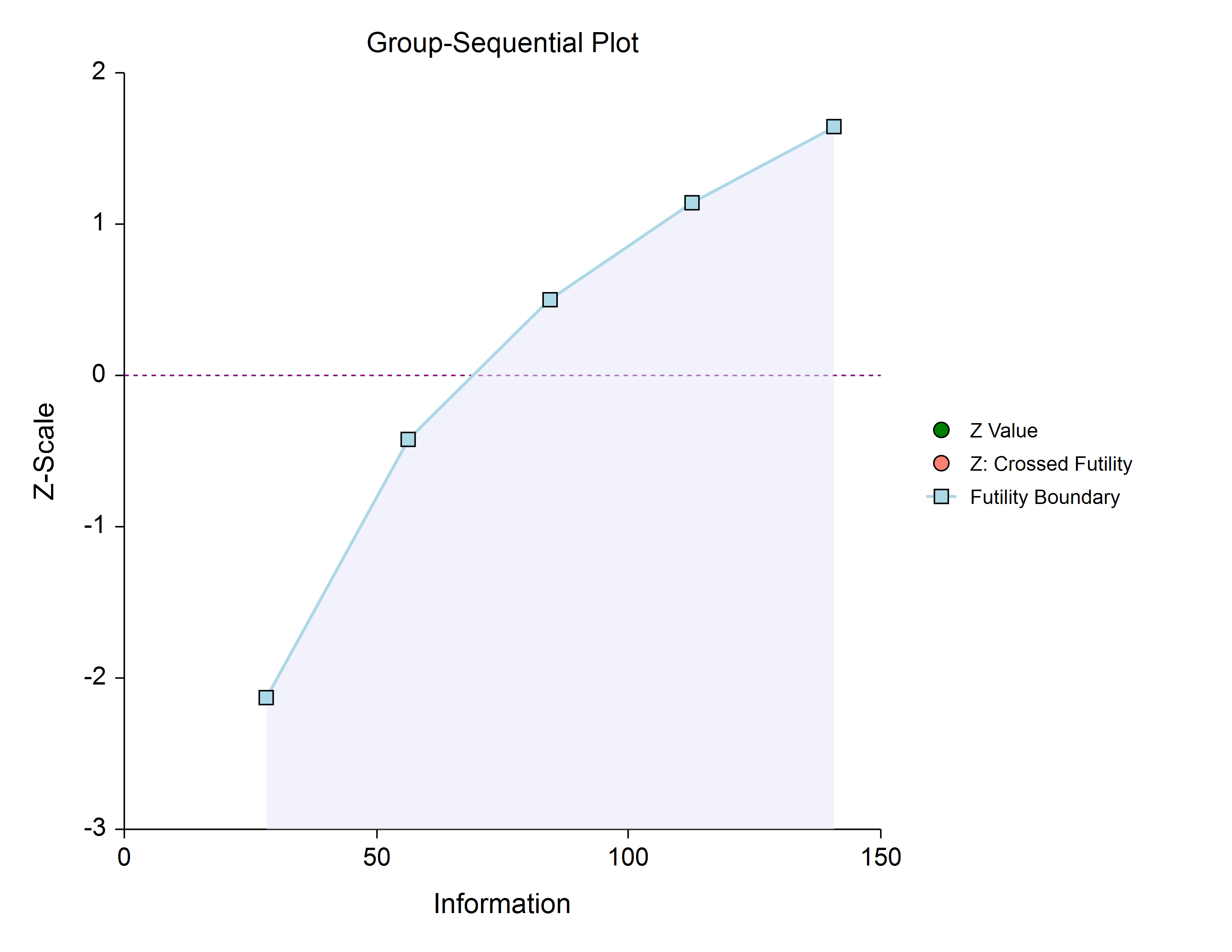
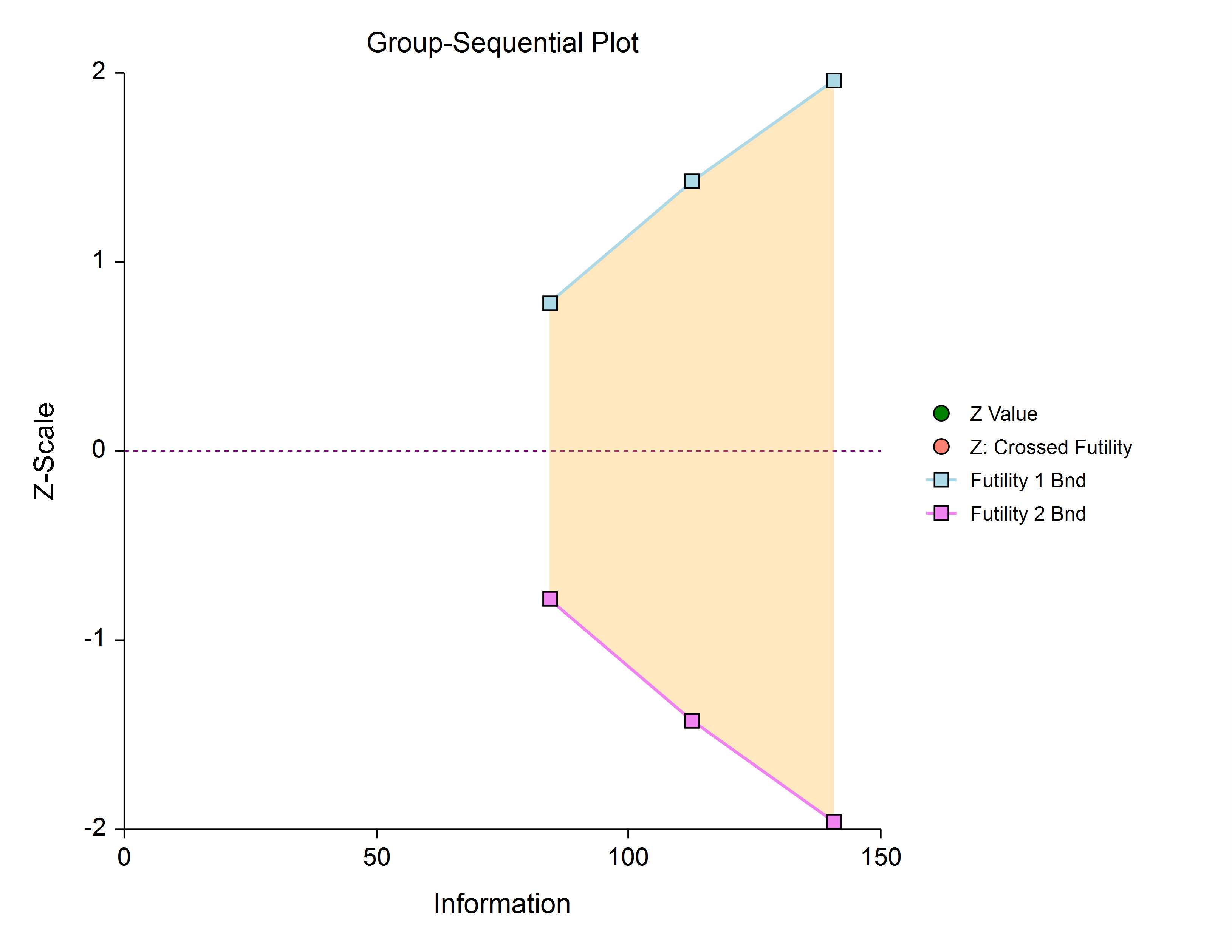
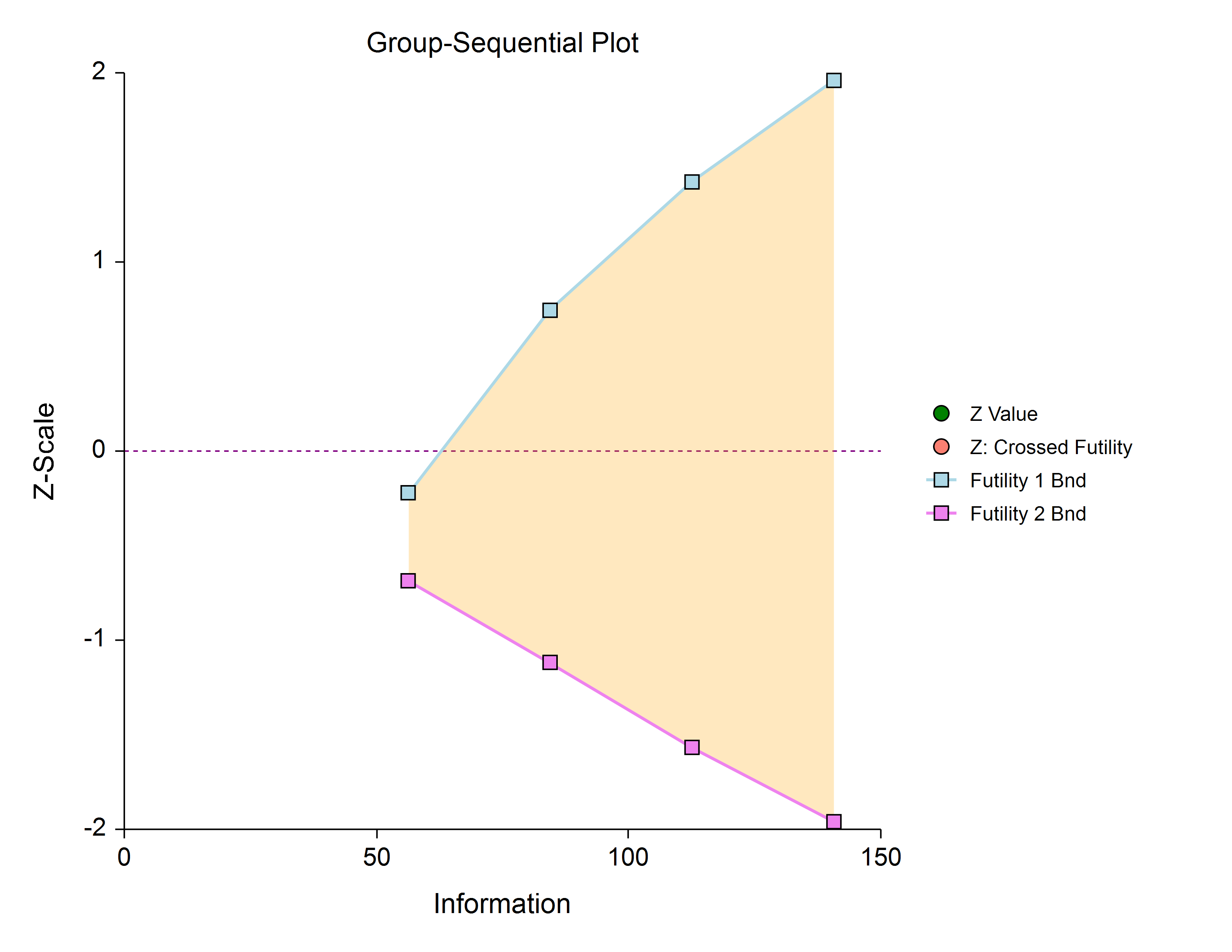
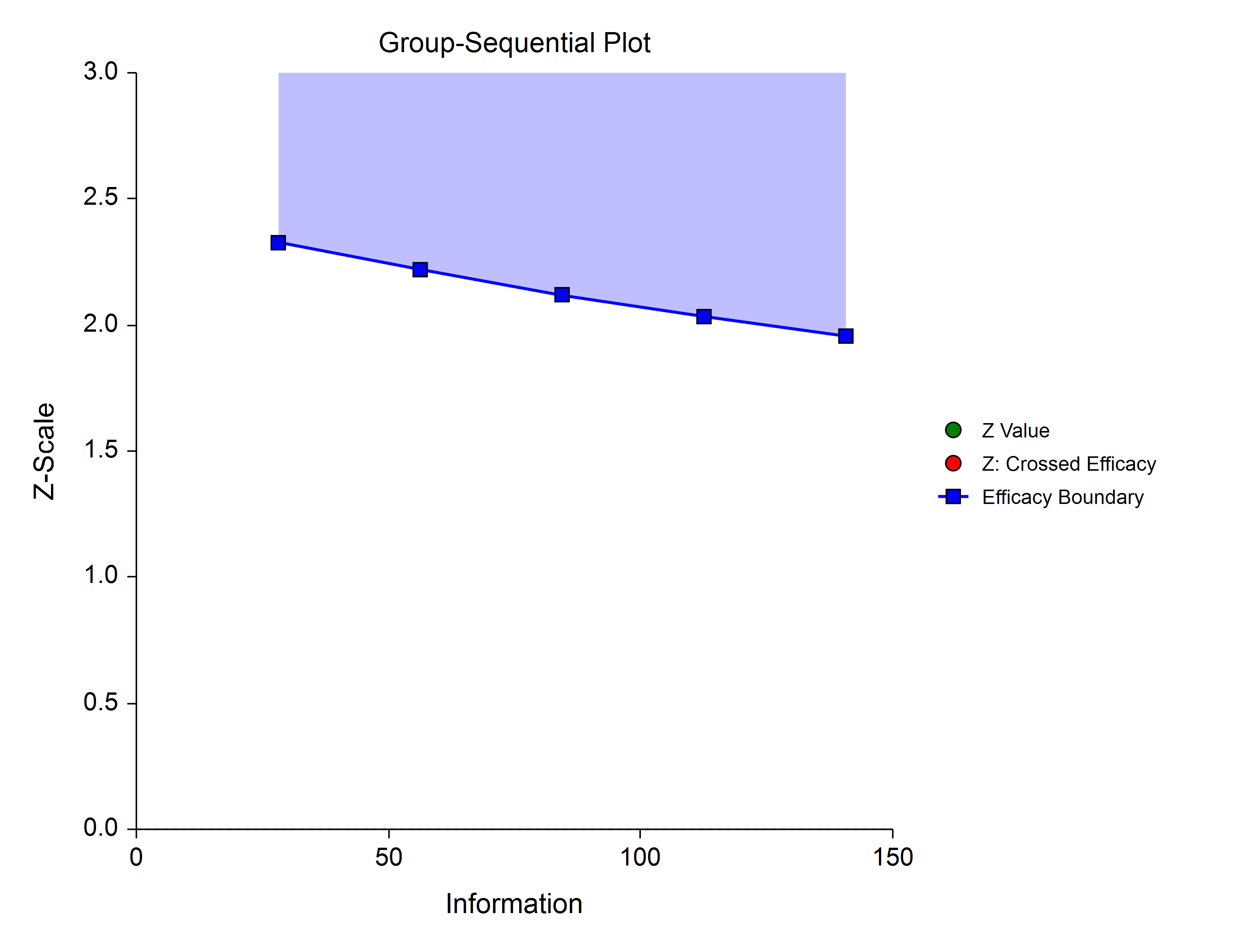
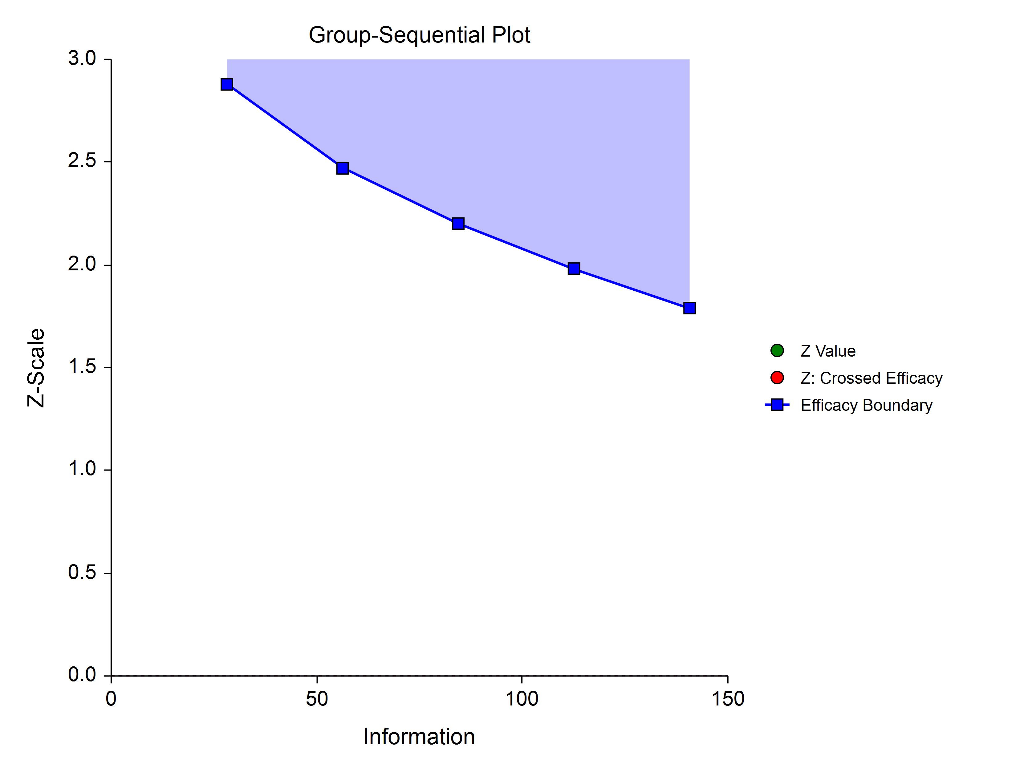
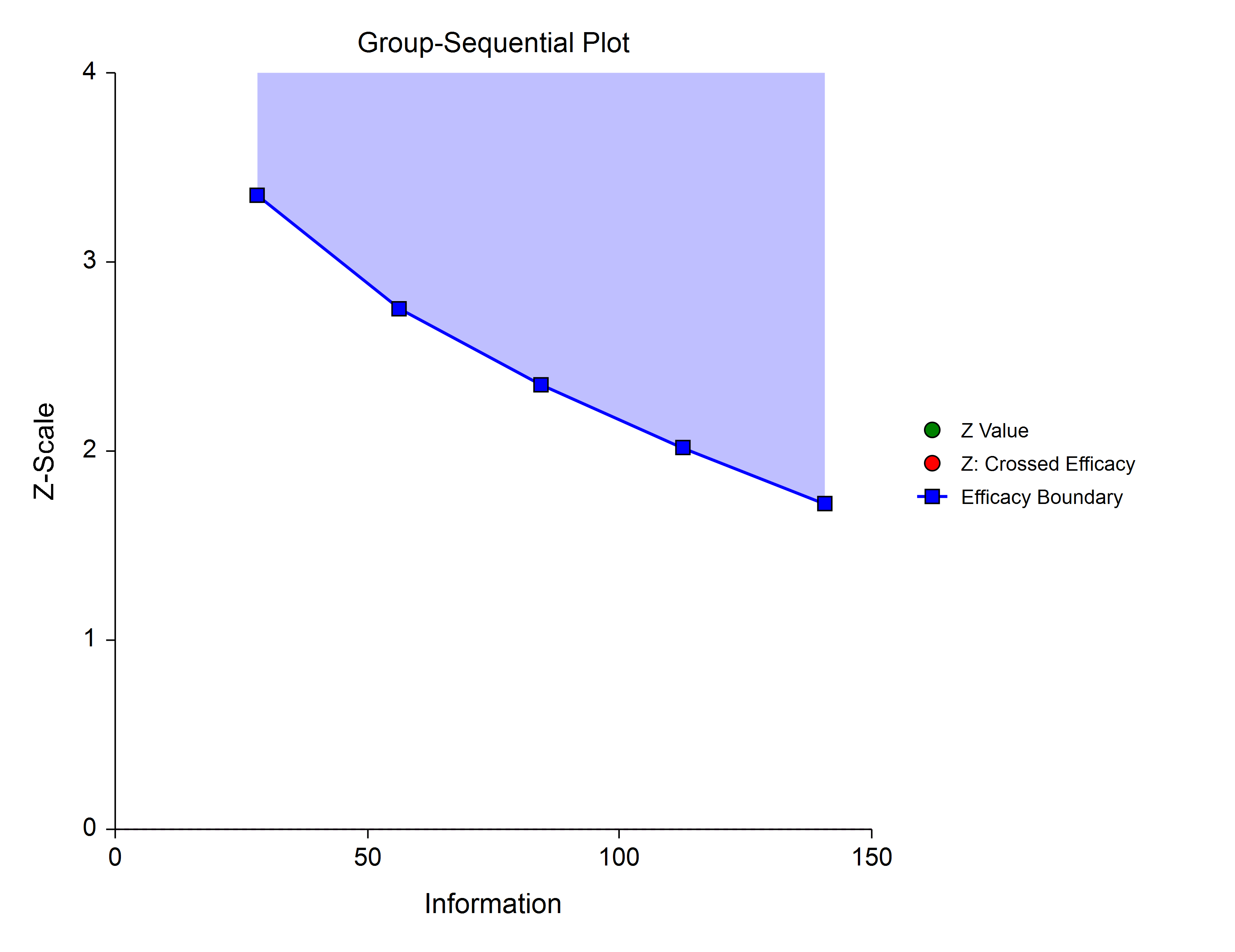
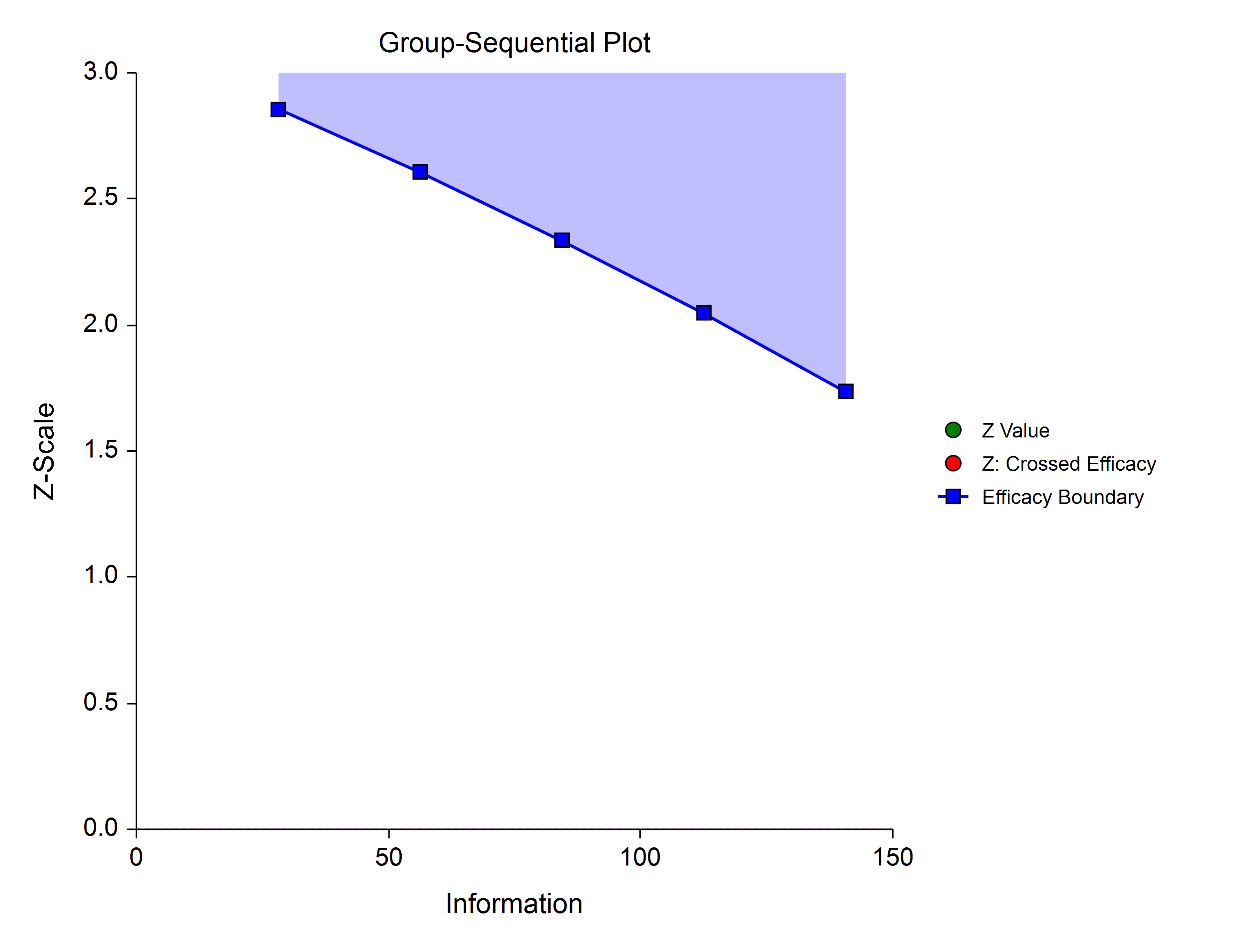
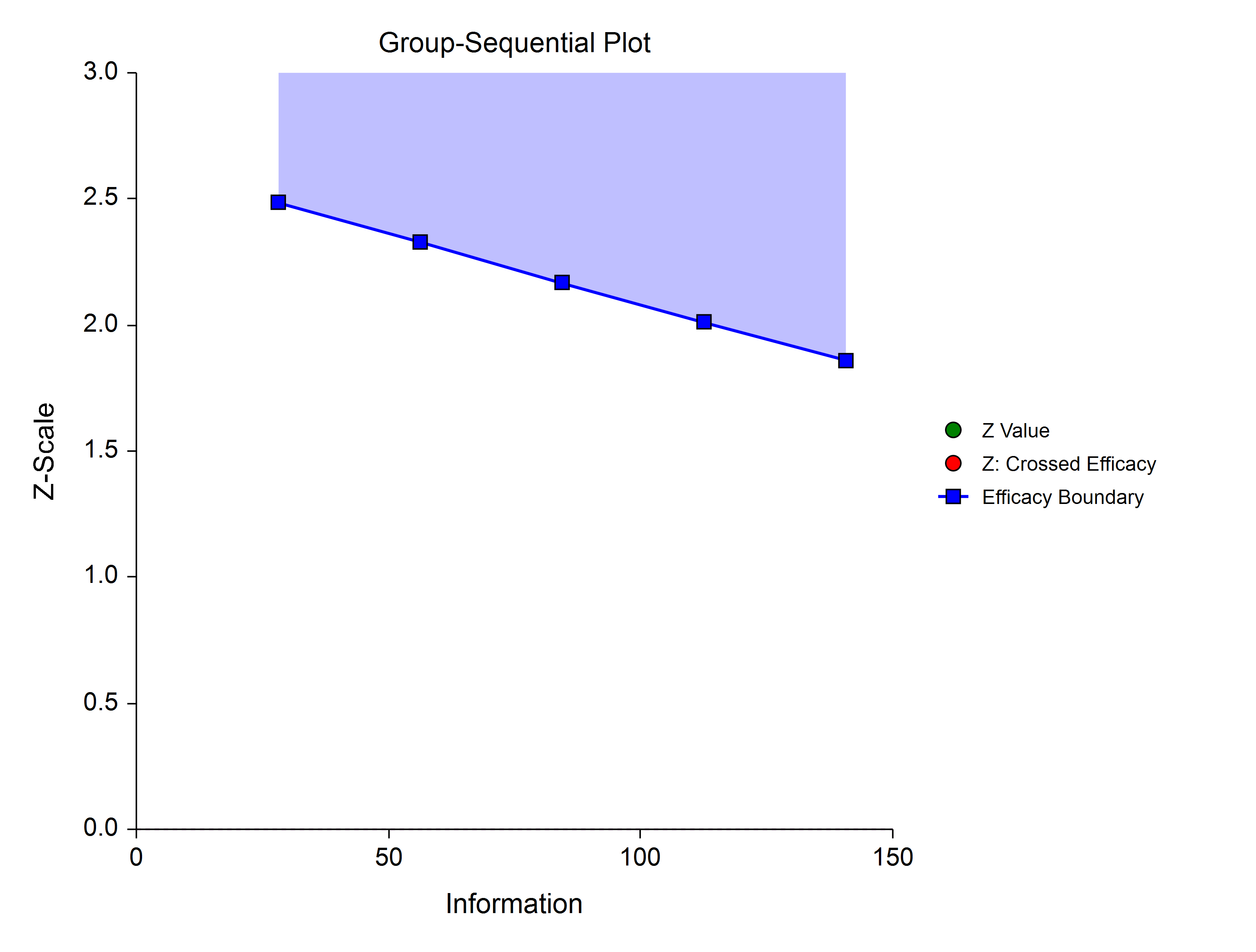
Each of these procedures can be used to determine power, sample size and/or boundaries for the corresponding group-sequential test. For one- and two-sided tests, efficacy and/or futility boundaries can be generated. The spacing of the stages can be equal or custom specified. Individual stages may also be skipped. Boundaries can be computed based on popular alpha- and beta-spending functions (O’Brien-Fleming Analog, Pocock Analog, Hwang-Shih-DeCani Gamma family, linear) or custom spending functions, or boundaries may be input directly, if desired. Futility boundaries can be binding or non-binding. Corresponding P-Value boundaries are given for each boundary statistic. Alpha and/or beta spent at each stage is reported. Plots of boundaries are also produced. Each procedure is used as the planning tool for determining sample size and initial boundaries. Stage data, as it is obtained, can be evaluated using the companion group-sequential analysis procedure in NCSS Statistical Analysis and Graphics software. The companion procedure also gives the option for sample-size re-estimation and updated boundaries for current-stage information. In that procedure, simulation can be used to evaluate boundary-crossing probabilities given the current stage results. 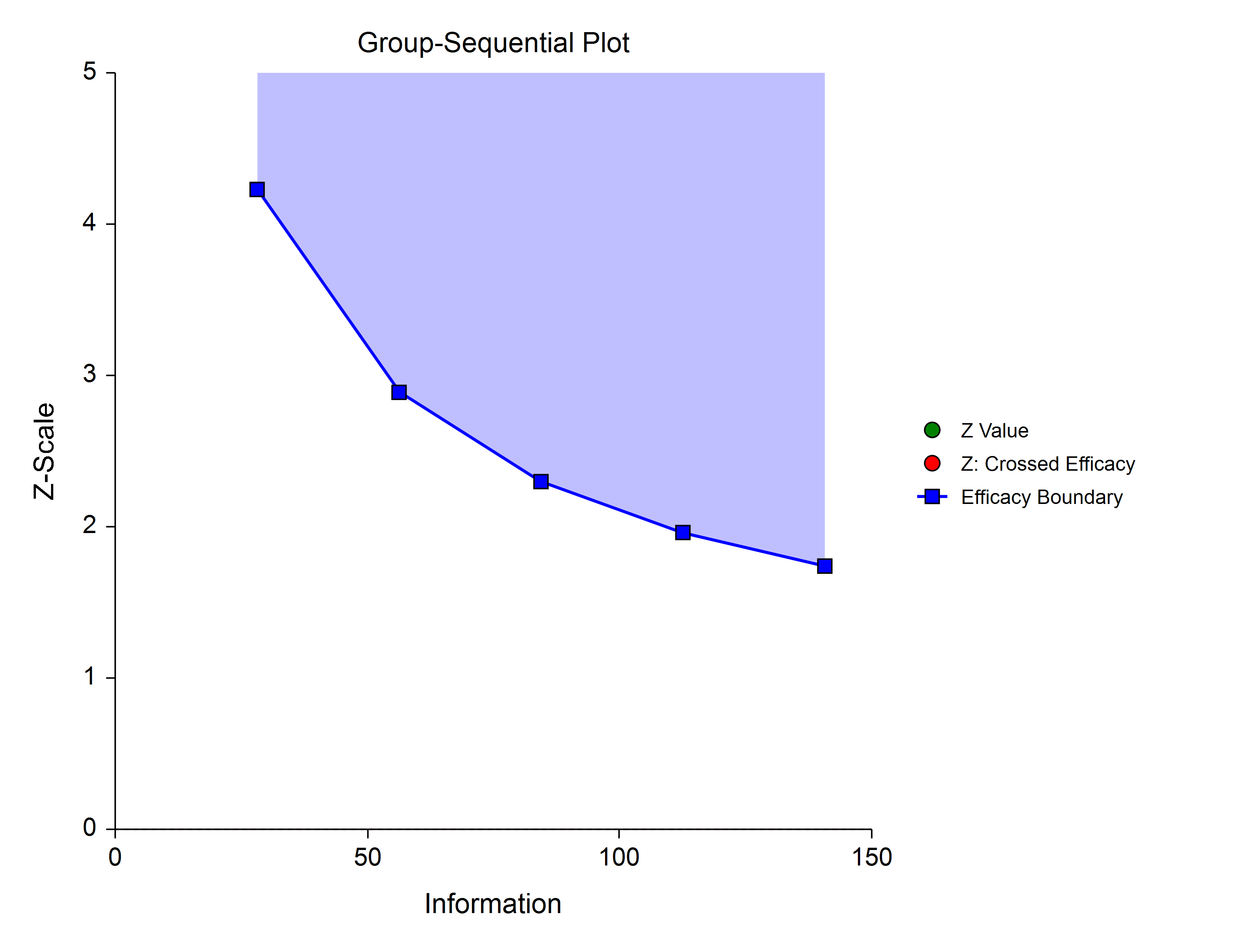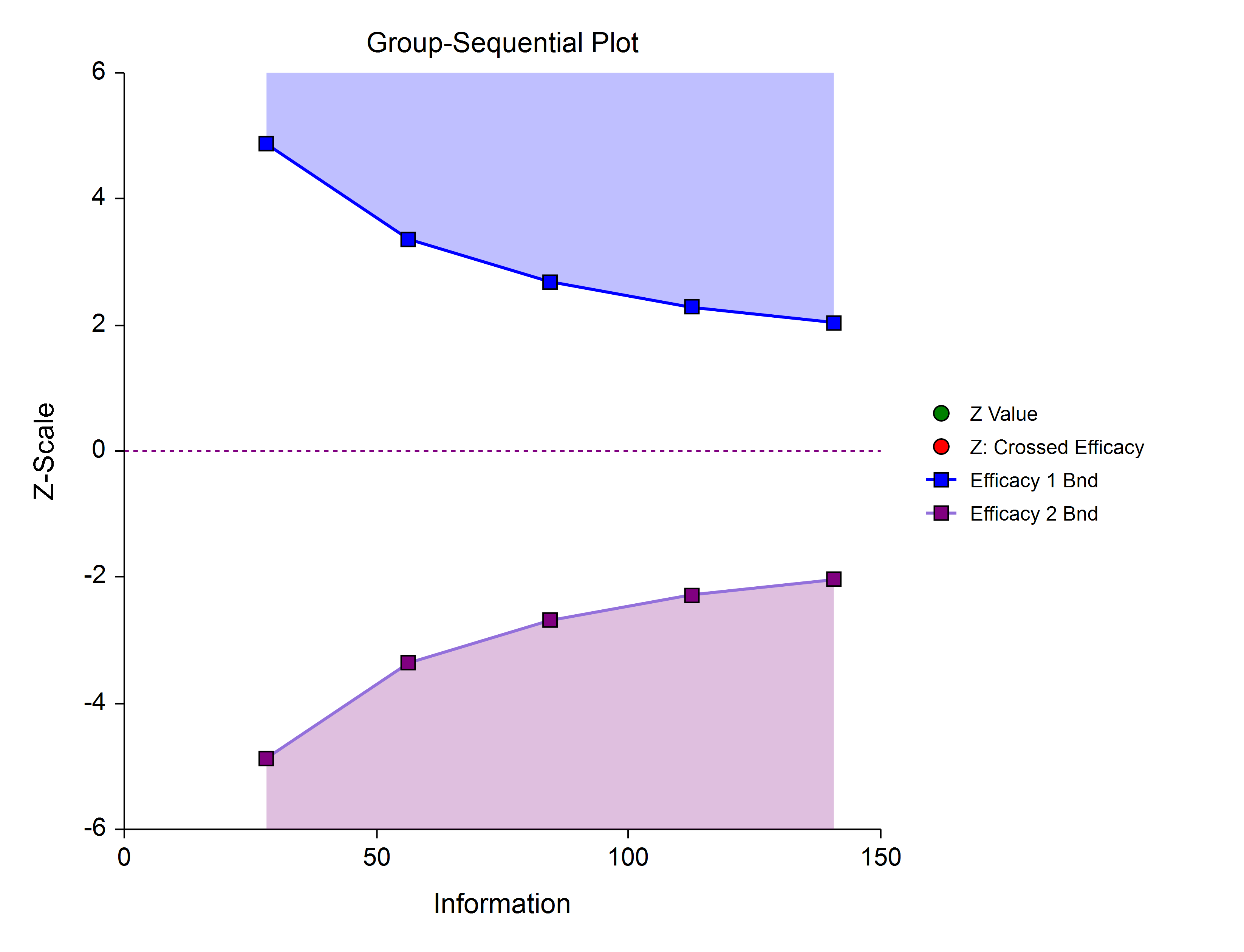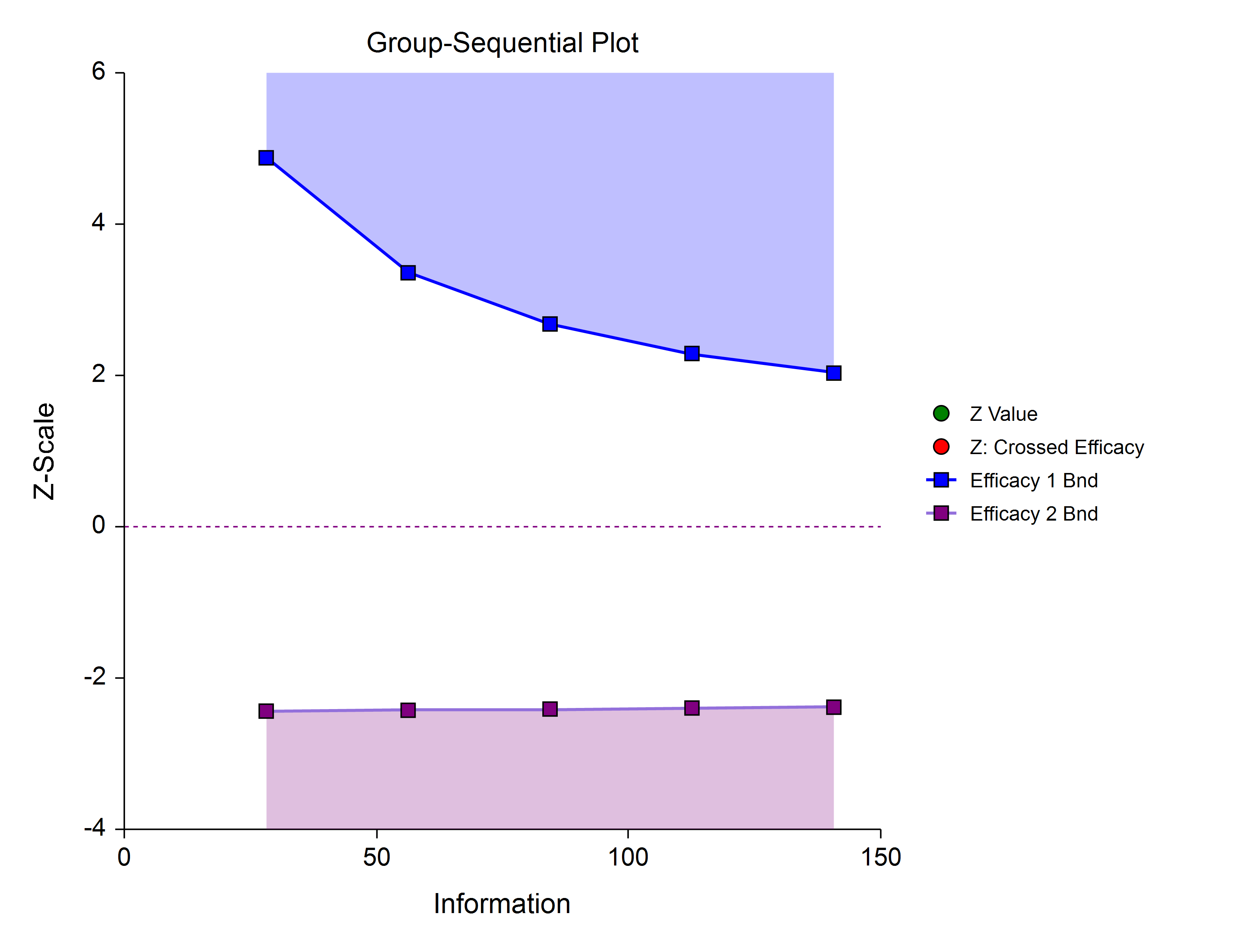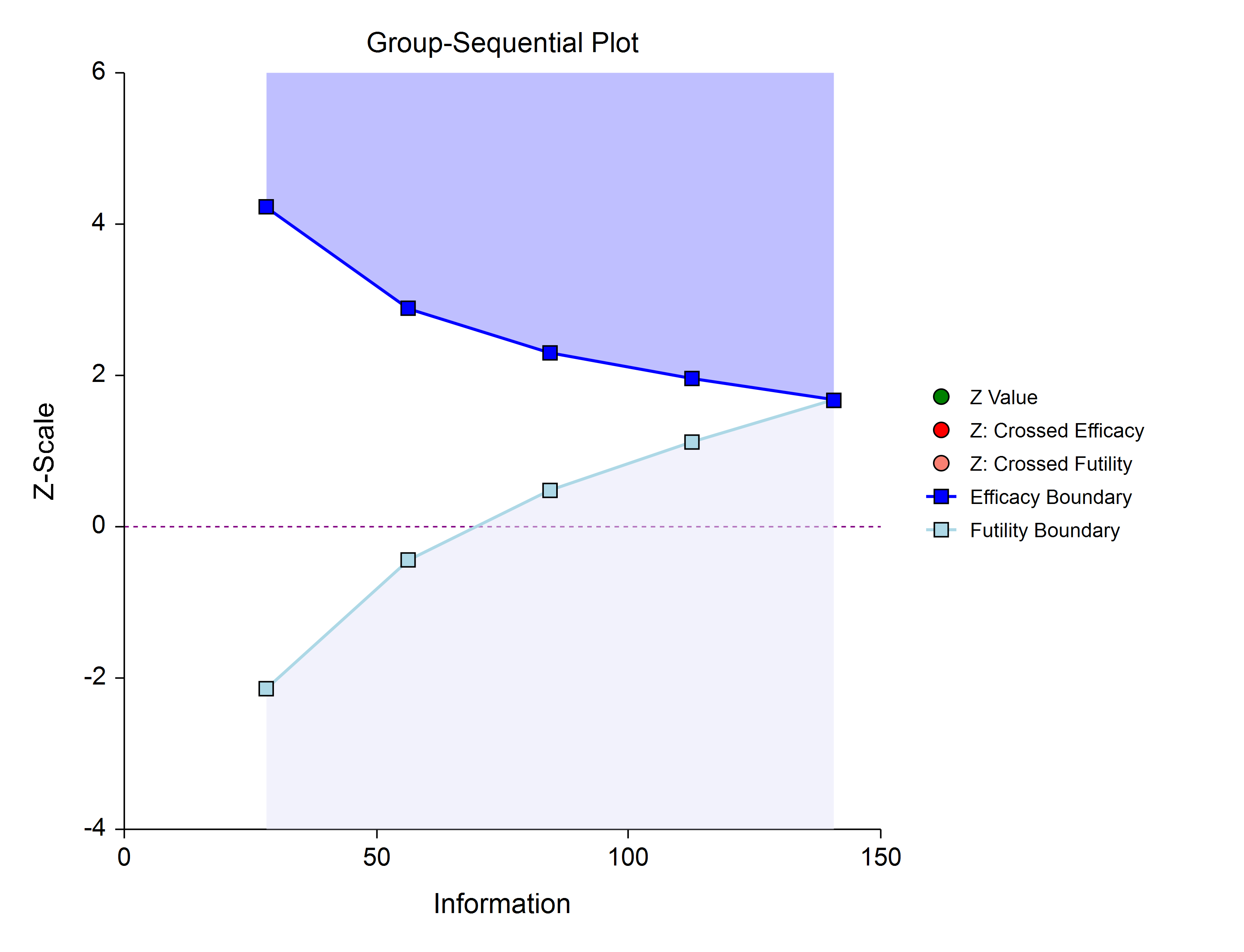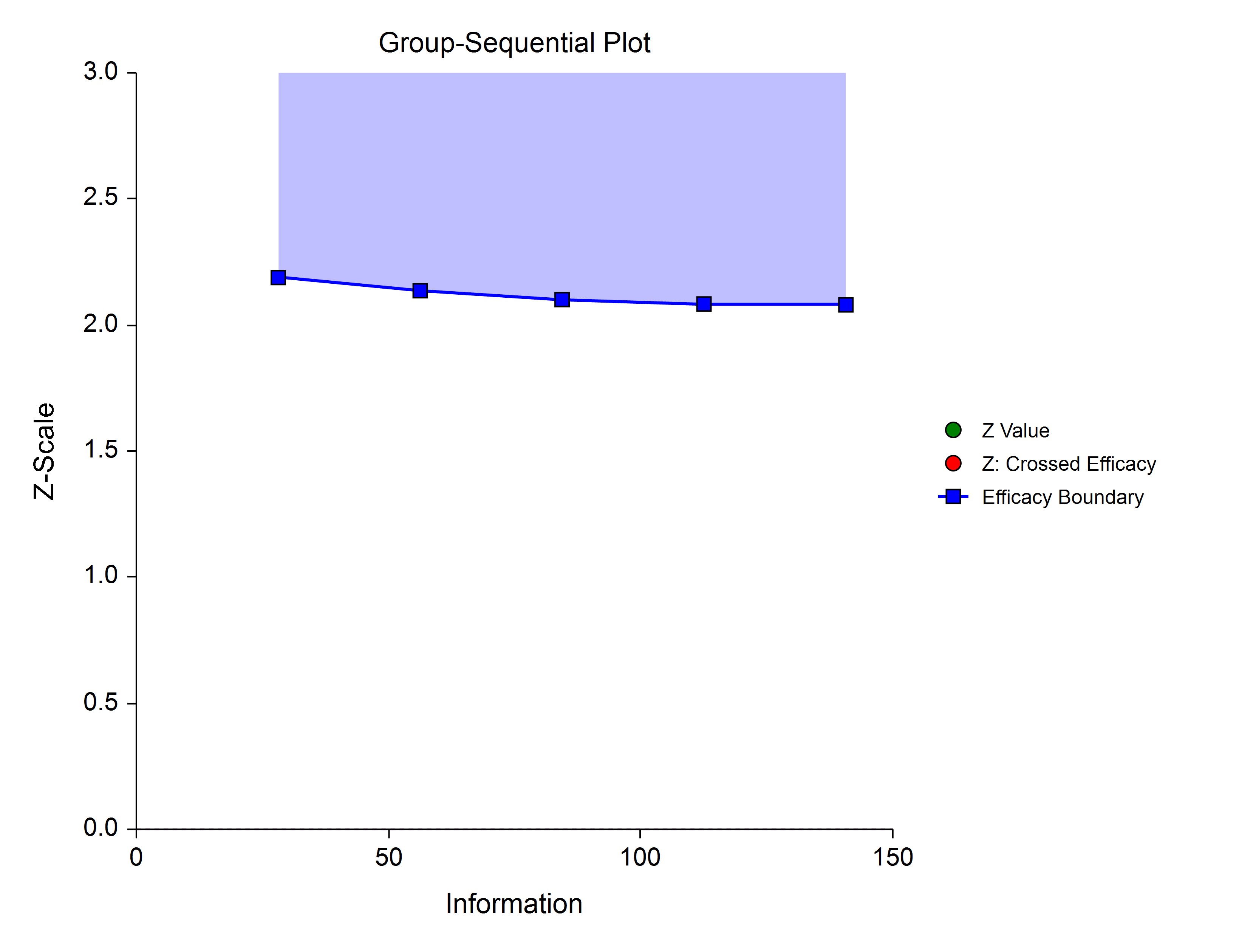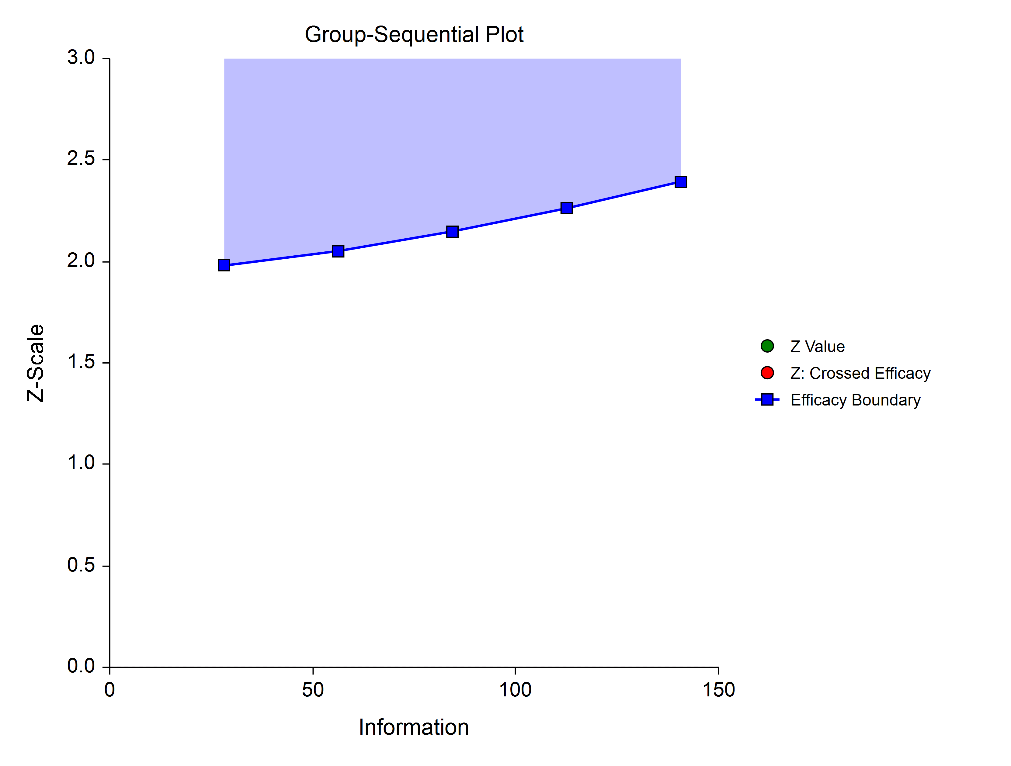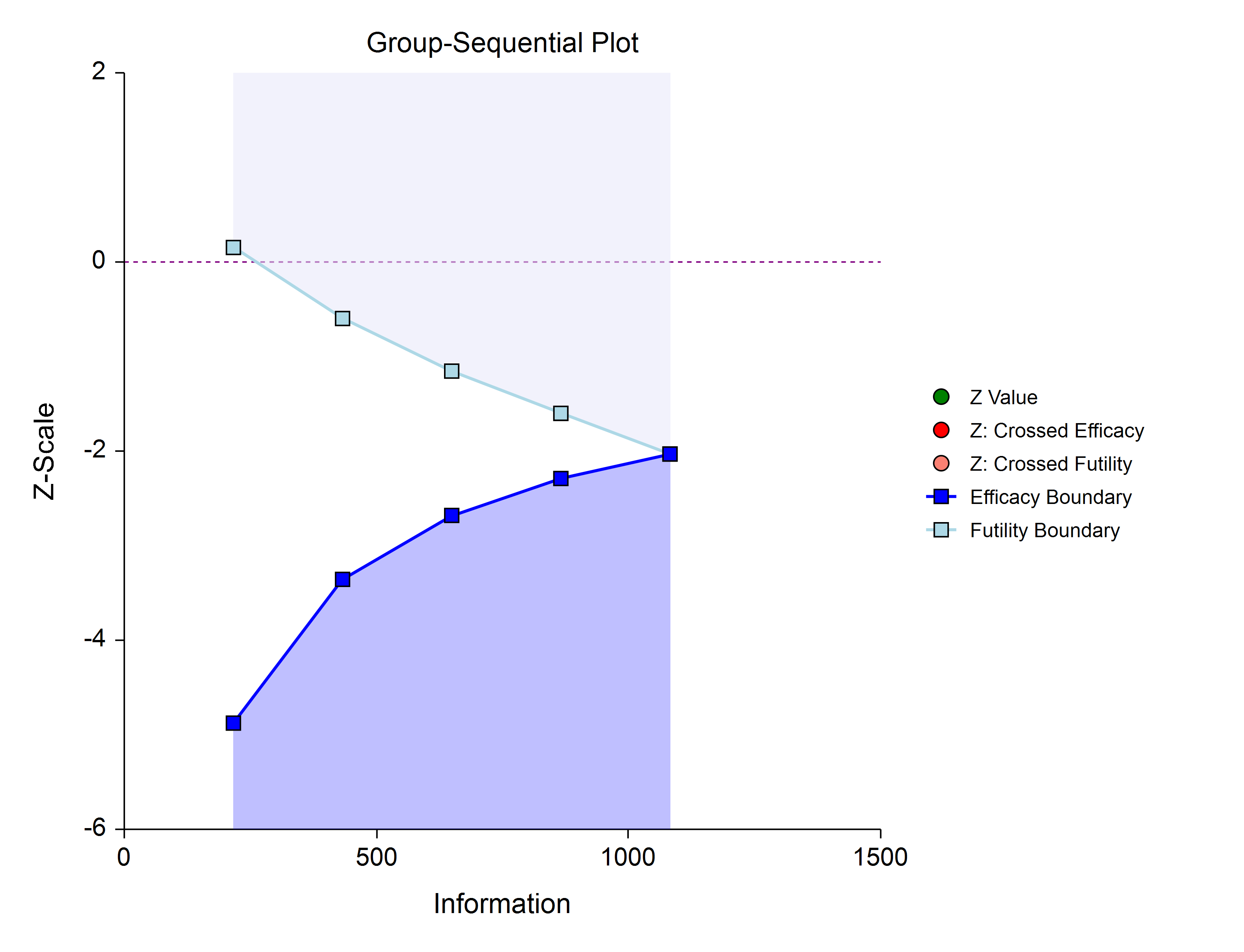An example of a group-sequential boundary plot produced in these procedures is shown below.

Outline of a Group-Sequential Study

There are three basic phases of a group-sequential (interim analysis) study:

1. Design
2. Group-Sequential Analysis
3. Reporting

Design Phase – Determine the Number of Subjects

To begin the group-sequential testing process, an initial calculation should be made to determine the sample size and target information if the final stage is reached (maximum information). The sample size calculation requires the specification of the following:

1. Alpha
2. Power
3. Test Direction (two-sided or one-sided direction)
4. Types of boundaries (efficacy, binding futility, non-binding futility)
5. Maximum number of stages
6. Proportion of maximum information at each stage
7. Spending functions
8. Effect Size Parameters

The design phase calculation is performed in the PASS group-sequential procedures. PASS software permits the user to easily try a range of effect size parameters (means, standard deviations, proportions, hazard rates), as these aren't always known in advance. The resulting sample size of the sample size calculation also permits the calculation of the maximum information, which is the total information of the study if the final stage is reached. Based on the maximum information, the target information and target sample size of each stage may be calculated. In particular, this permits the user to have a target sample size for the first stage.

Group-Sequential Analysis Phase

A group sequential analysis consists of a series of stages where a decision to stop or continue is made at each stage. This analysis can be performed using the companion (analysis) procedure to this sample size procedure, in NCSS.

First Interim Stage

The design phase gives the target number of subjects for the first stage. The study begins, and response data is collected for subjects, moving toward the first-stage target number of subjects, until a decision to perform an analysis on the existing data is made. The analysis at this point is called the first stage. Unless the number of subjects at the first stage matches the design target for the first stage, the calculated information at the first stage will not exactly match the design information for the first stage. Further, the sample parameter estimates will rarely, if ever, match the parameters used in the calculation of the information at the design stage, and thus the calculated information at the first stage will differ from the design information. Generally, the calculated information will not differ too greatly from the design information, but regardless, spending function group-sequential analysis is well-suited to make appropriate adjustments for any differences. The first stage information is divided by the maximum information to obtain the stage one information proportion (or information fraction). This information proportion is used in conjunction with the spending function(s) to determine the alpha and/or beta spent at that stage. In turn, stage one boundaries, corresponding to the information proportion, are calculated. A z-(or t-)statistic is calculated from the raw data values. The stage one statistic is compared to each of the stage one boundaries. Typically, if one of the boundaries is crossed, the study is stopped (non-binding futility boundaries may be an exception).

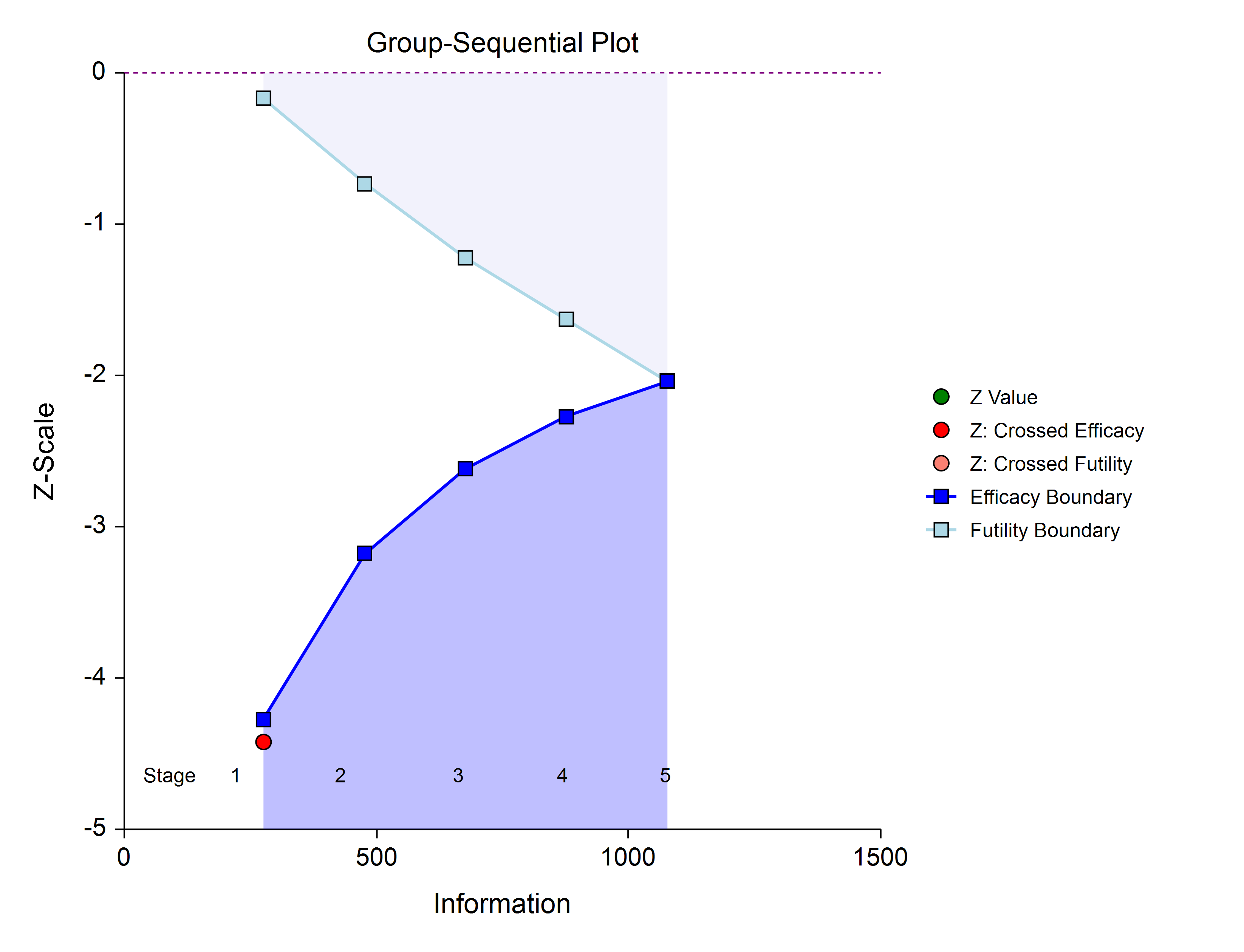
If none of the boundaries are crossed the study continues to the next stage.

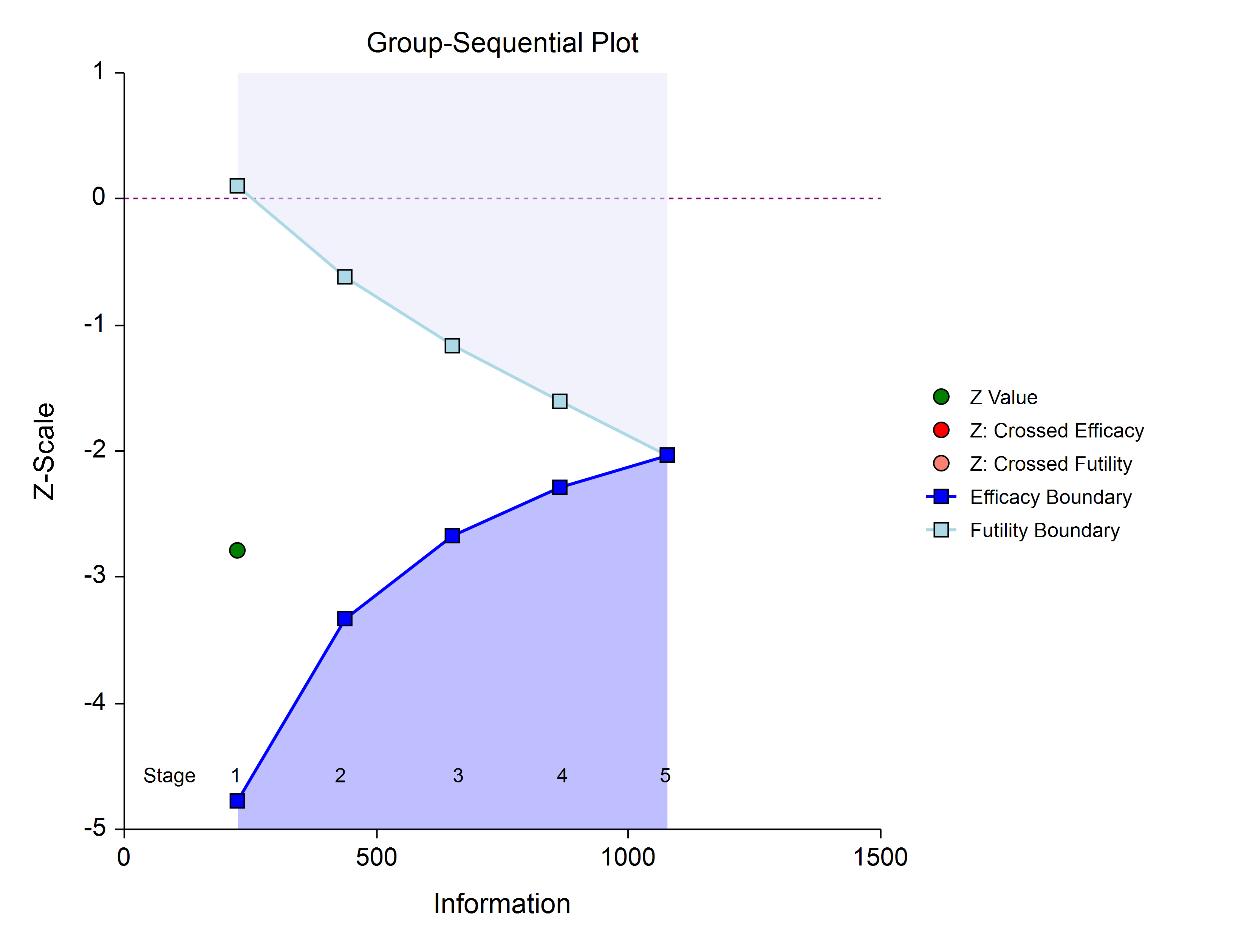
If none of the boundaries are crossed it may also be useful to examine the conditional power or stopping probabilities of future stages, using the NCSS procedure. Conditional power and stopping probabilities are based on the user-specified supposed true difference.

Second and other interim stages (if reached)

Since the first stage information proportion is not equal to the design information proportion, a designation must be made at this point as to the target information of the second stage. Two options are available in the NCSS procedure. One option is to target the information proportion of the original design. For example, if the original design proportions of a four-stage design are 0.25, 0.50, 0.75, 1.0, and the stage one observed proportion is 0.22, the researcher might still opt to target 0.50 for the second stage, even though that now requires an additional information accumulation of 0.28 (proportion). The third and fourth stage targets would also remain 0.75 and 1.0. A second option is to adjust the target information proportionally to the remaining proportions. For this option, if the design proportions are 0.25, 0.50, 0.75, 1.0, and 0.22 is observed, the remaining 0.78 is distributed proportionally to the remaining stages. In this example, the remaining target proportions become 0.48, 0.74, 1.0. For either option, once the target information is determined for the next stage, revised target sample sizes are given (in the NCSS procedure), and the study continues until the decision is made to perform the next interim analysis on the cumulative response data. In the same manner as the first stage, the current stage information proportion is used with the spending function to determine alpha and/or beta spent at the current stage. The current stage boundaries are then computed. The z-statistic is calculated and compared to the boundaries, and a decision is made to stop or continue. If a boundary is crossed, the study is typically stopped.

If none of the boundaries are crossed the study continues to the next stage.

Once again, if no boundary is crossed, conditional power and stopping probabilities may be considered based on a choice of a supposed true difference. The study continues from stage to stage until the study is stopped for the crossing of a boundary, or until the final stage is reached.

Final Stage (if reached)

The final stage (if reached) is similar to all the interim stages, with a couple of exceptions. For all interim analyses the decision is made whether to stop for the crossing of a boundary, or to continue to the next stage. At the final stage, only the decision of efficacy or futility can be made. Another intricacy of the final stage that does not apply to the interim stages is the calculation of the maximum information. At the final stage, the current information must become the maximum information, since the spending functions require that the proportion of information at the final look must be 1.0. If the current information at the final stage is less than the design maximum information, the scenario is sometimes described as under-running. Similarly, if the current information at the final stage is greater than the design maximum information, the result may be termed over-running. For both under-running and over-running, the mechanism for adjustment is the same, and is described in the Technical Details section, under Information and Total Information. Aside from these two exceptions, the final stage analysis is made in the same way that interim analyses were made. The remaining alpha and beta to be spent are used to calculate the final stage boundaries. If the test is a one-sided test, then the final stage boundary is a single value. The final stage z-statistic is computed from the sample proportions of the complete data from each group. The z-statistic is compared to the boundary and a decision of efficacy or futility is made.

Reporting Phase

Once a group-sequential boundary is crossed and the decision is made to stop, there remains the need to properly summarize and communicate the study results. Some or all of the following may be reported:

1. Boundary plot showing the crossed boundary
2. Adjusted confidence interval and estimate of the proportion difference
3. Sample size used

Boundary plot showing the crossed boundary

The boundary plot gives an appropriate visual summary of the process leading to the reported decision of the study.

Adjusted confidence interval and estimate of the proportion difference

Due to the bias that is introduced in the group-sequential analysis process, the raw data confidence interval of the difference in proportions should not be used. An adjusted confidence interval should be used instead.

Sample size used

The sample size at the point the study was stopped should be reported in addition to the sample size that would have been used had the final stage been reached.

Technical Details

Many articles and texts have been written about group sequential analysis. Details of many of the relevant topics are discussed below, but this is not intended to be a comprehensive review of group-sequential methods. One of the more influential works in the area of group-sequential analysis is Jennison and Turnbull (2000).

Null and Alternative Hypotheses

The null and alternative hypotheses for group-sequential tests are the same as those of standard one-stage tests, with alternative hypothesis options of one- or two-sided tests.

Stages in Group-Sequential Testing

The potential to obtain the benefit from a group-sequential design and analysis occurs when the response data are collected over a period of weeks, months, or years rather than all at once. A typical example is the case where patients are enrolled in a study as they become available, as in many types of clinical trials. A group-sequential testing stage is a point in the accumulation of the data where an interim analysis occurs, either by design or by necessity. At each stage, a test statistic is computed with all the accumulated data, and it is determined whether a boundary (efficacy or futility) is crossed. When an efficacy (or futility) boundary is crossed, the study is usually concluded, and inference is made. If the final stage is reached, the group-sequential design forces a decision of efficacy or futility at this stage. For the discussions below, a non-specific interim analysis stage is referenced as k, and the final stage is K.

Test Statistic

The z-statistic (or t-statistic) for any stage k is obtained from all the accumulated data up to and including that stage.

Group-Sequential Design Phase

In most group-sequential studies there is a design or planning phase prior to beginning response collection. In this phase, researchers specify the anticipated number and spacing of stages, the types of boundaries that will be used, the desired alpha and power levels, the spending functions, the anticipated parameter values, and an estimate of the true difference. Based on these input parameters, an initial set of boundaries is produced, an estimate of the total number of needed subjects is determined, and the anticipated total information at the final stage is calculated. This procedure can be used to make these planning phase sample size estimation calculations.

Information and Total Information

In the group-sequential design phase, the information at any stage k may be calculated from the specified parameter values (for variance) and the sample sizes. When the analysis is carried out, the sample estimates will be used in place of parameter values for variance calculations. The final stage (K) or total (design) information is calculated from the appropriate parameter estimates and the final sample sizes. The proportion of the total information (or information fraction) at any stage is the ratio of the current stage information to the total information. The information fractions are used in conjunction with the spending function(s) to define the alpha and/or beta to be spent at each stage. However, if the final stage is reached, the final stage information will likely be larger or smaller than the total information used in planning. When the final stage information is larger than the total information used in planning, it is called over-running. When the final stage information is smaller than the total information used in planning, it is called under-running. In either case, the spending function is adjusted to accommodate the inequality. See the discussion in Wassmer and Brannath (2016), pages 78-79, or Jennison and Turnbull (2000), pages 153-154, 162.

Types of Boundaries

A variety of boundary designs are available to reflect the needs of the study design.

Efficacy Only (One-Sided)

The simplest group-sequential test involves a single set of stage boundaries with early stopping for efficacy.

Efficacy Only (Two-Sided, Symmetric)

This boundary type would be used if the goal is to compare treatments, and it is not known in advance which treatment should be better.

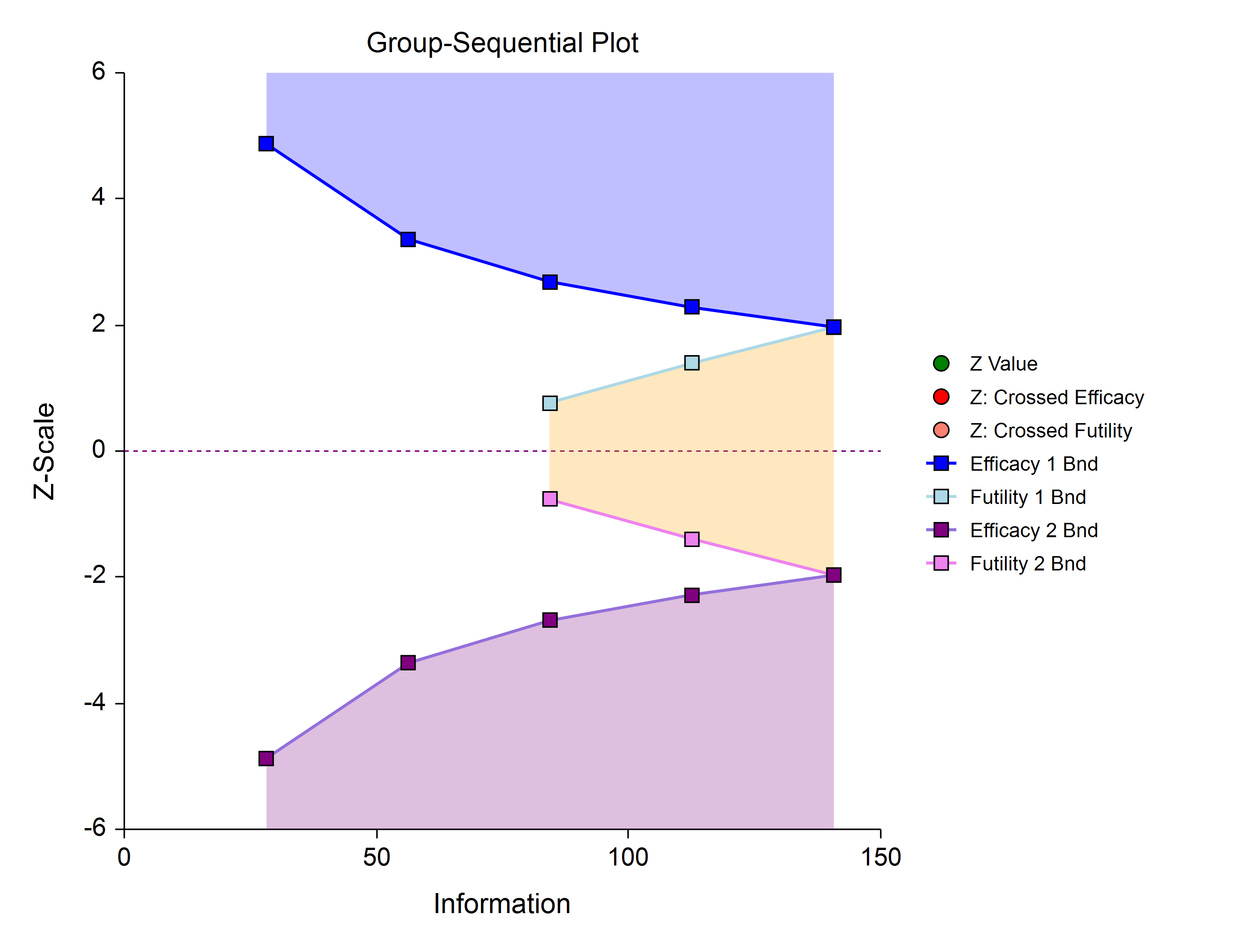
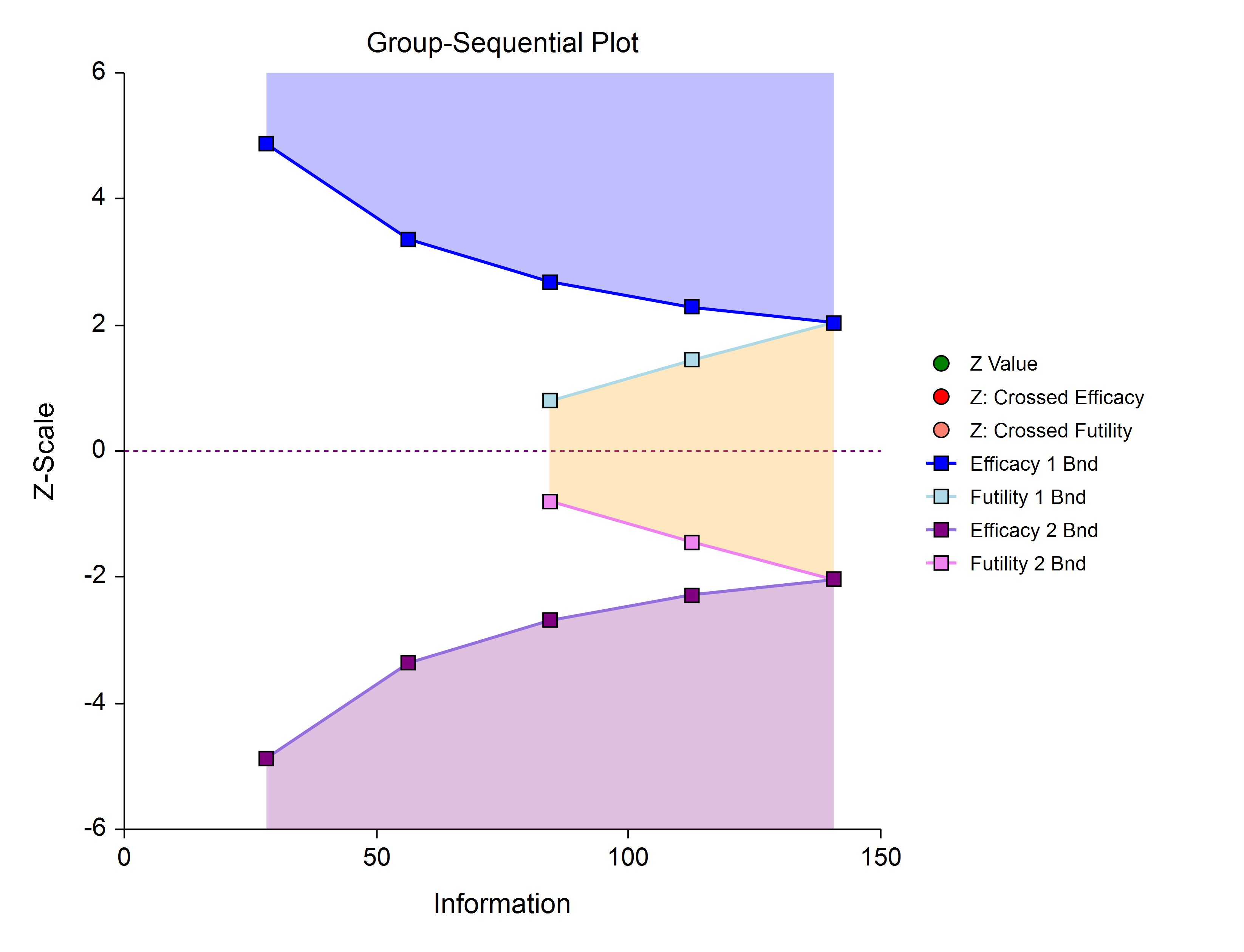
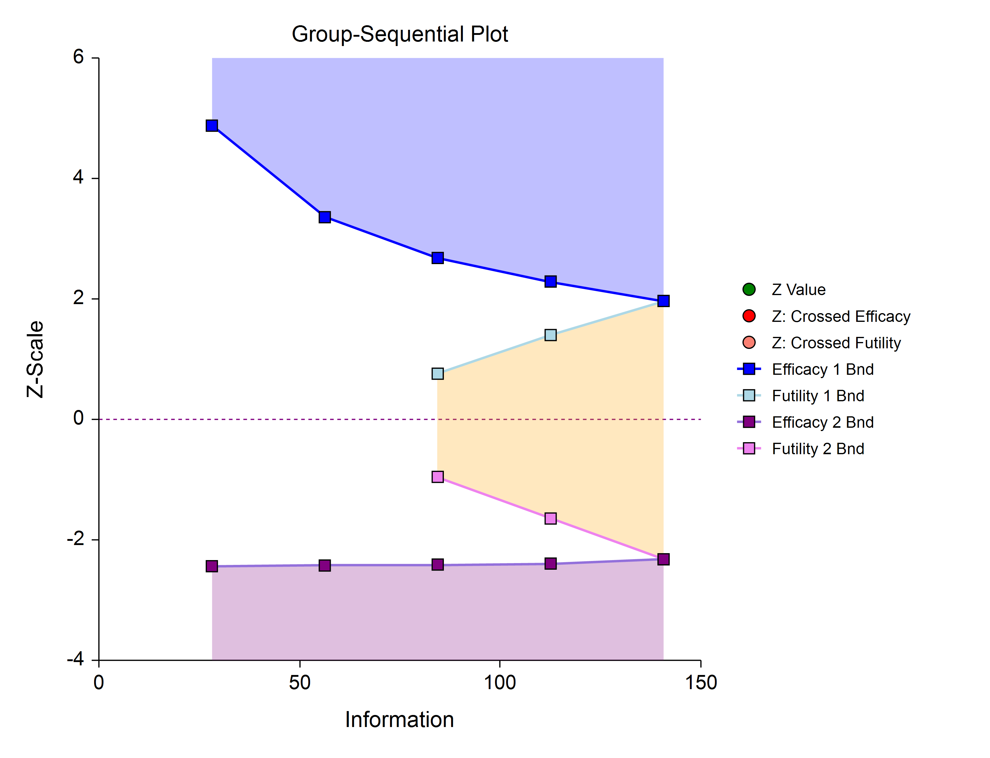
Efficacy 1 and Efficacy 2 / Harm (Two-Sided, Asymmetric)

These boundaries might be used to show efficacy on one side or harm on the other side. This design might be used in place of a one-sided efficacy and futility design if showing harm has additional benefit over stopping early for futility.

Efficacy and Binding Futility (One-Sided)

This design allows early stopping for either efficacy or futility. For binding futility designs, the Type I error protection (alpha) is only maintained if the study is strictly required to stop if either boundary is crossed.

Efficacy and Non-Binding Futility (One-Sided)

This design also allows early stopping for either efficacy or futility. For non-binding futility designs, the Type I error protection (alpha) is maintained, regardless of whether the study continues after crossing a futility boundary. However, the effect is to make the test conservative (alpha is lower than the stated alpha and power is lower than the stated power).

Efficacy and Binding Futility (Two-Sided, Symmetric)

This design allows early stopping for either efficacy or futility on either side. Alpha is preserved only if crossing of futility boundaries strictly leads to early stopping for futility. In early looks of this design, the futility boundaries may overlap. Overlapping futility boundaries may be skipped or left as they are.

Efficacy and Non-Binding Futility (Two-Sided, Symmetric)

This design allows early stopping for either efficacy or futility on either side. Alpha is preserved even when the study is allowed to continue after crossing a futility boundary. In early looks of this design, the futility boundaries may overlap. Overlapping futility boundaries may be skipped or left as they are.

Efficacy 1, Efficacy 2 / Harm, and Binding Futility (Two-Sided, Asymmetric)

This design allows early stopping for efficacy and efficacy futility, and for harm and harm futility (or efficacy 2 and efficacy 2 futility). Binding futility boundaries require that the study is stopped when a binding futility boundary is crossed. In early looks of this design, the futility boundaries may overlap. Overlapping futility boundaries may be skipped or left as they are.

Efficacy 1, Efficacy 2 / Harm, and Non-Binding Futility (Two-Sided, Asymmetric)

This design allows early stopping for efficacy and efficacy futility, and for harm and harm futility (or efficacy 2 and efficacy 2 futility). Non-binding futility boundaries do not require that the study is stopped when a binding futility boundary is crossed, but the study design is conservative. In early looks of this design, the futility boundaries may overlap. Overlapping futility boundaries may be skipped or left as they are.

Futility Only (One-Sided)

In this design, the interim analyses are used only for futility. Please be aware that, due to computational complexity, these boundaries may take several minutes to compute, particularly when some stages are skipped.

Futility Only (Two-Sided, Symmetric)

In this design, the study is stopped early only for futility. Overlapping futility boundaries may be skipped or left as they are. Please be aware that, due to computational complexity, these boundaries may take several minutes to compute, particularly when overlapping boundaries are removed or some stages are skipped.

Futility Only (Two-Sided, Asymmetric)

In this design, all stages previous to the final stage are used only for futility. Overlapping futility boundaries may be skipped or left as they are. Please be aware that, due to computational complexity, these boundaries may take several minutes to compute, particularly when overlapping boundaries are removed or some stages are skipped.

Boundary Calculations

The foundation of the spending function approach used in these procedures is given in Lan & DeMets (1983). These procedures implement the methods given in Reboussin, DeMets, Kim, & Lan (1992) to calculate the boundaries and stopping probabilities of the various group sequential designs. Some adjustments are made to these methods to facilitate the calculation of futility boundaries.

Binding vs. Non-Binding Futility Boundaries

Futility boundaries are used to facilitate the early stopping of studies when early evidence leans to lack of efficacy. When binding futility boundaries are to be used, the calculation of the futility and efficacy boundaries assumes that the study will be strictly stopped at any stage where a futility or efficacy boundary is crossed. If strict adherence is not maintained, then the Type I and Type II error probabilities associated with the boundaries are no longer valid. One (perhaps undesirable) effect of using binding futility boundaries is that the resulting final stage boundary may be lower than the boundary given in the corresponding fixed-sample design. When non-binding futility boundaries are calculated, the efficacy boundaries are first calculated ignoring futility boundaries completely. This is done so that alpha may be maintained whether or not a study continues after crossing a futility boundary. One (perhaps undesirable) effect of using non-binding futility boundaries is that the overall group-sequential test becomes conservative (alpha is lower than the stated alpha and power is lower than the stated power).

Spending Functions

Spending functions are used to distribute portions of alpha (or beta) to the stages according to the proportion of accumulated information at each look.

Spending Function Characteristics

1. Spending functions give a value of zero when the proportion of accumulated information is zero.
2. Spending functions are increasing functions.
3. Spending functions give a value of alpha (or beta) when the proportion of accumulated information is one.

Using spending functions in group-sequential analyses is very flexible in that neither the information proportions nor the number of stages need be specified in advance to maintain Type I and Type II error protection.

Spending Functions Available in this Procedure

The following spending functions are shown as alpha-spending functions. The corresponding beta-spending function is given by replacing α with β.

O’Brien-Fleming Analog

The O’Brien Fleming Analog (Lan & DeMets, 1983) roughly mimics the O’Brien-Fleming (non-spending function) design, with the key attribute that only a small proportion of alpha is spent early. Its popularity comes from it proportioning enough alpha to the final stage that the final stage boundary is not too different from the fixed-sample (non-group-sequential) boundary.

Pocock Analog

The Pocock Analog (Lan & DeMets, 1983) roughly mimics the Pocock (non-spending function) design, with the key attribute that alpha is spent roughly equally across all stages.

Power Family

The power family of spending functions has a ρ parameter that gives flexibility in the spending function shape. A power family spending function with a ρ of 1 is similar to a Pocock design, while a power family spending function with a ρ of 3 is more similar to an O’Brien-Fleming design.

ρ = 1

ρ = 2

ρ = 3

Hwang-Shih-DeCani (Gamma Family)

The Hwang-Shih-DeCani gamma family of spending function has a γ parameter that allows for a variety of spending functions.

γ = -3

γ = -1

γ = 1

γ = 3

Using Simulation to obtain Boundary Crossing Probabilities

In addition to providing an overall estimate of power, it can be useful to researchers to know the probability of crossing each of the group-sequential boundaries, given a specified assumed value for the proportions. The following steps are used to estimate these probabilities using simulation: 1. Determine the target (cumulative) sample sizes for each stage, including the final stage. Fractional sample sizes are rounded up to the next integer. 2. For each simulation, obtain a simulated data set with the final stage sample sizes. Simulated values are generated from Bernoulli distributions with user-specified proportions. 3. Determine whether simulation Z-values are ‘held out’ after crossing a boundary, or whether simulation Z-values are ‘left in’ (compared to boundaries at all future stages, regardless of whether a boundary was crossed at a previous stage). a. If simulation Z-values are ‘held out’ after crossing a boundary, it is determined for each simulation which boundary was crossed first (except in the case of non-binding futility boundaries). b. If simulation Z-values are ‘left in’ after crossing a boundary, it is determined for each simulation all the boundaries where the Z-value is across the boundary. 4. The proportion of simulations crossing each boundary provides an estimate of the probability of crossing each boundary, given the specified assumed proportions. 5. Overall power and alpha calculations are also based on the specification of ‘held out’ or ‘left in’. a. When Hold Out is selected, power and alpha are calculated as the sum of all efficacy boundary proportions. b. When Leave In is selected, power and alpha are calculated as the efficacy boundary proportion of the final stage.

Non-binding Futility Boundaries

When non-binding futility boundaries are used, the study may continue when a futility boundary is crossed. The simulation proportions will have a slightly different interpretation when this is the case.

An Example Setup and Output

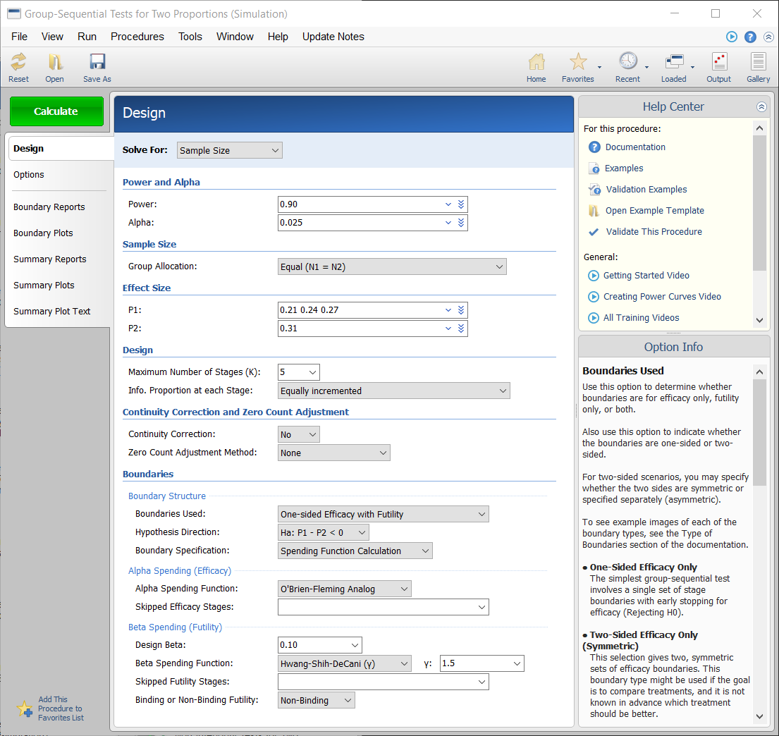
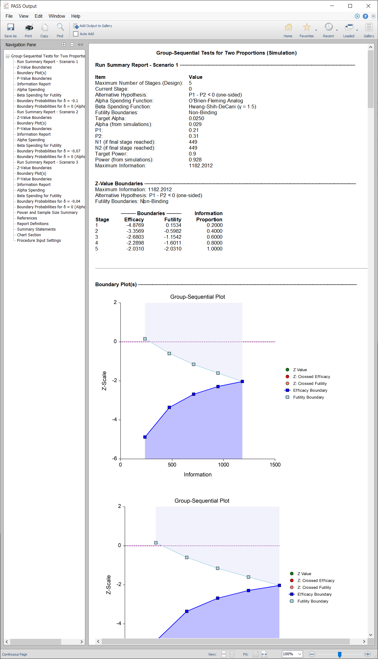
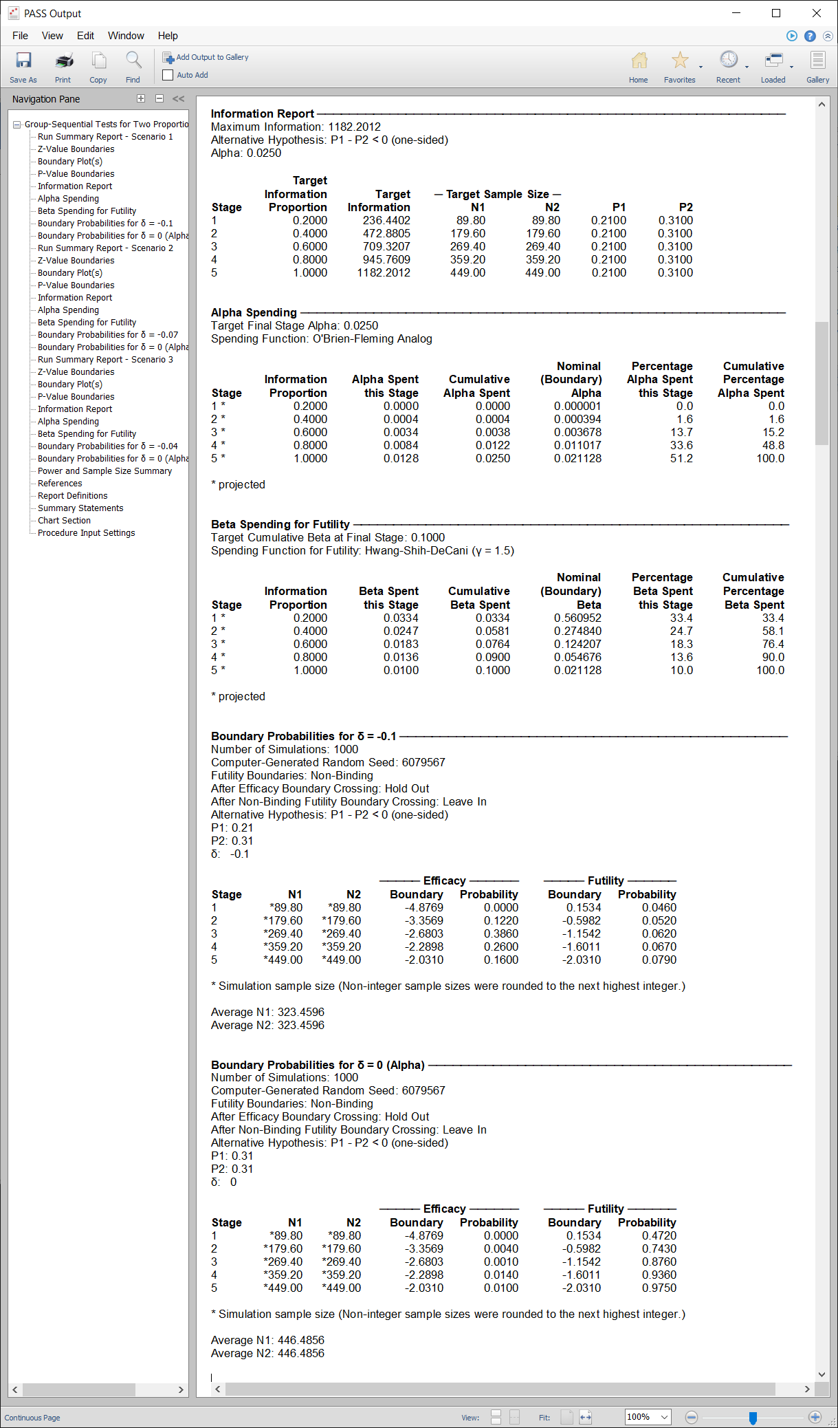
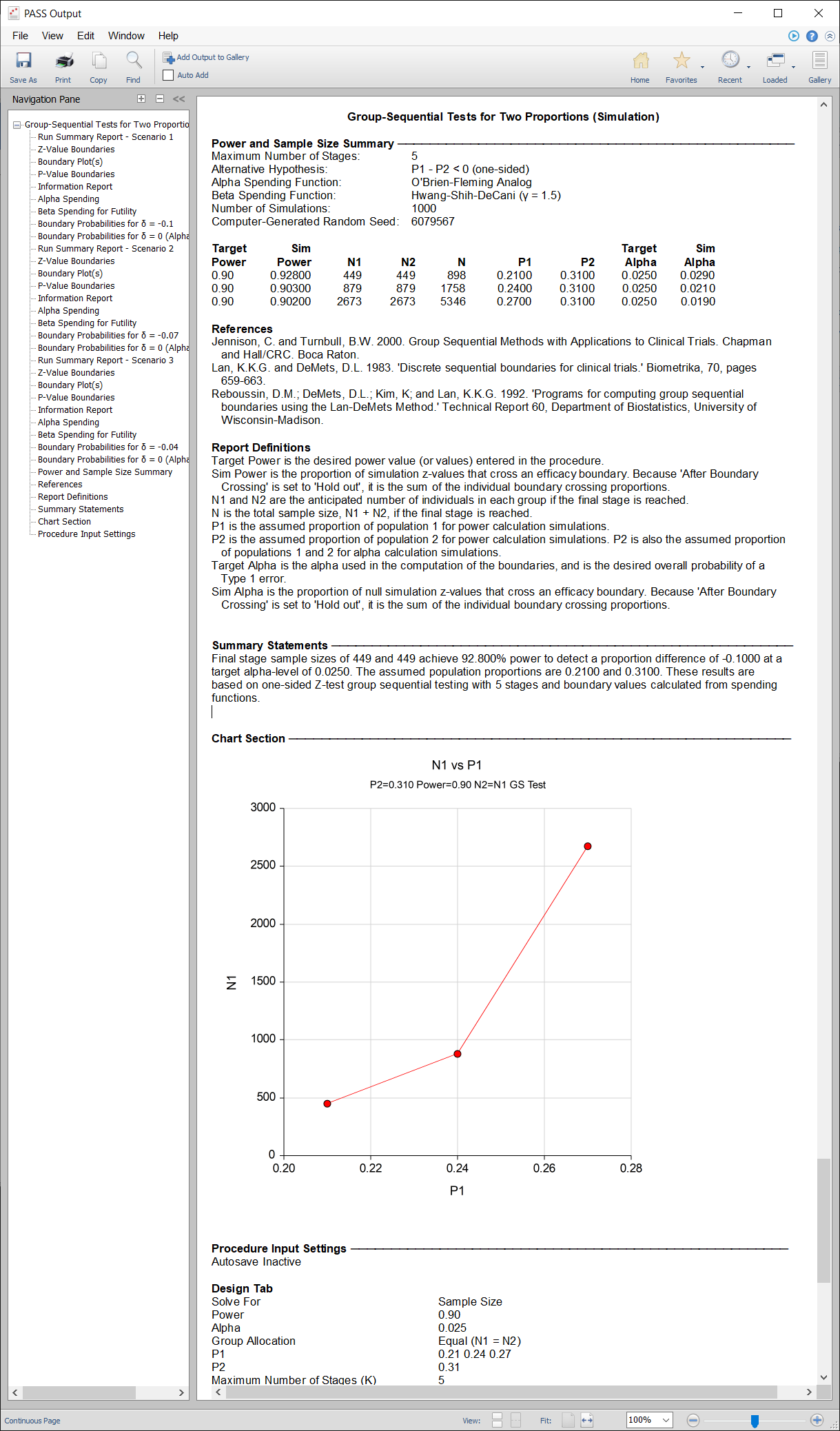
A childbirth study is to be conducted to determine whether a new approach during labor results in a lower proportion of C-sections than the standard techniques. The response for each patient is C-section or no C-section. A one-sided test with alpha equal to 0.025 is used. The Z-Test will use unpooled variance estimation with no continuity correction. The new approach is assigned to Group 1, and the standard is assigned to Group 2. The design calls for five equally spaced stages if the final stage is reached. A power of 0.90 is needed. The assumed caesarian proportion for the standard approach is 0.31. Researchers wish to examine the sample sizes needed for new approach proportions of 0.21, 0.24, and 0.27. Both efficacy and non-binding futility boundaries are intended. The efficacy (alpha-spending) spending function used is the O’Brien-Fleming analog. The Hwang-Shih-DeCani (Gamma) beta-spending function with gamma parameter 1.5 is used for futility.

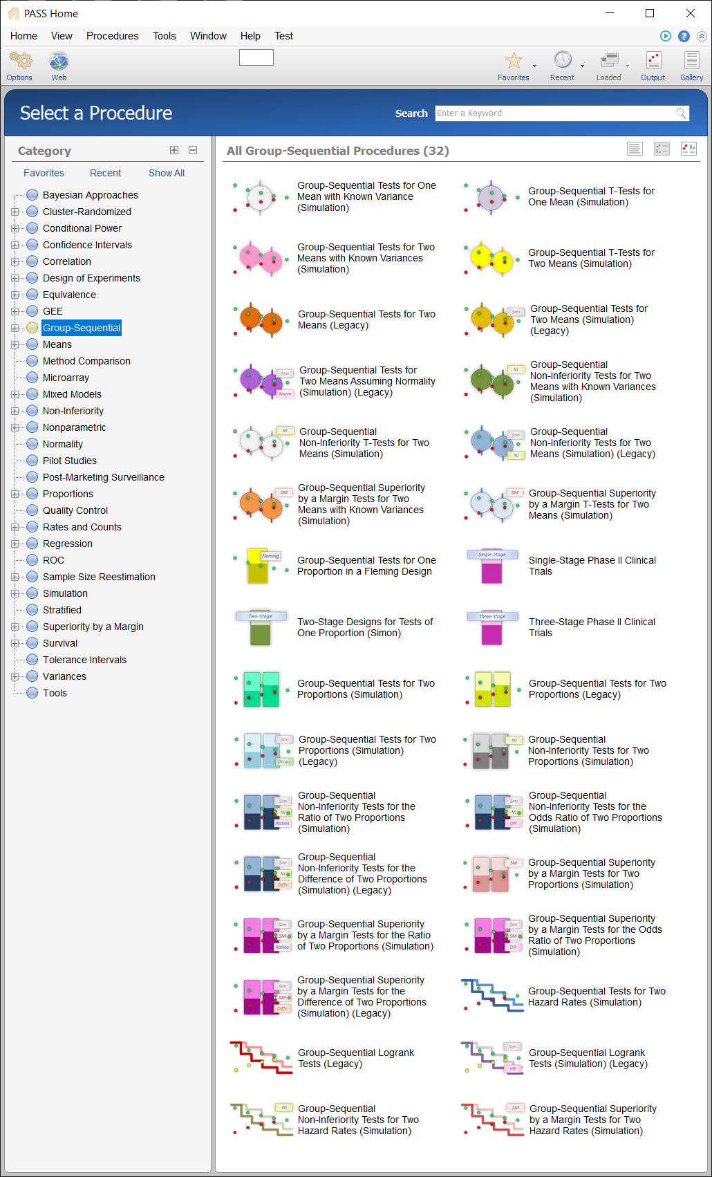
PASS Home Window - Group-Sequential Procedures

Procedure Window for Group-Sequential Tests for Two Proportions

PASS Output Window for Group-Sequential Tests for Two Proportions