Now Playing: Power and Sample Size Primer (12:17)
Description:
This video is intended to be a basic introduction or primer to the principles of power and sample size estimation. It begins with definitions, such as null and alternative hypotheses, test statistics, p-values, Type 1 and Type 2 errors, Alpha, Beta, and Power. The factors influencing power and sample size are then discussed, including some of the intricacies of specifying the population parameters. The video concludes with an example that relates these definitions and sample size considerations to a real-world setting. We begin with some basic definitions:
In the scope of this discussion, the null hypothesis is a statement of equality of a population parameter of interest to a specified value, or to some other population parameter or parameters. The null hypothesis is chosen such that rejection of the null hypothesis, based on evidence from the gathered data, will lead to an evidence-based conclusion of the alternative hypothesis. The alternative hypothesis is a statement of inequality of the population parameters of interest. Providing evidence in favor of the alternative hypothesis by providing evidence against the null hypothesis is at the heart of statistical research methods. Typical research methods dictate that the null and alternative hypotheses should be determined in advance of the study, in particular before the data have been viewed.
The collected data are summarized by a single statistic about the parameter of interest. This statistic is commonly called the test statistic. The test statistic is compared to a known distribution of the possible values of the test statistic, assuming the null hypothesis is true. A p-value is calculated based on the test statistic, which reflects the probability of obtaining that test statistic, or one more extreme, if the null hypothesis is true. Small p-values indicate low probability of obtaining such a test statistic if the null hypothesis is true, and therefore, evidence against the null hypothesis. Similarly, large p-values indicate test statistics consistent with data obtained under the null hypothesis, and thus, lack evidence against the null hypothesis.
It is common practice to set a value, such that if the p-value turns out to be lower than this cutoff value, it will be determined that the evidence is strong enough to reject the null hypothesis, and favor or conclude the alternative hypothesis. This cutoff value is called Alpha. It is very common for journals, departments, and/or guidelines to prescribe a required alpha for a particular type of study or statistical test in that field.
Since the truth about the population from which samples are obtained is unknown, and because of the variation inherent to sampling, two types of errors can be made when making a conclusion about the null hypothesis. First, one may reject the null hypothesis when it is true. This is called a Type 1 Error. The probability of a Type 1 Error is Alpha. Second, one may fail to reject the null hypothesis when it is indeed false. This is called a Type 2 Error. The probability of a Type 2 Error is called Beta. It is easy to see that researchers would like to put limits on the likelihood of Type 1 and Type 2 errors, as these result in the wrong conclusion entirely.
Because Alpha limits the probability of rejection of the null hypothesis, setting Alpha simultaneously sets the probability of committing a Type I error.
Instead of specifying Beta for a planned study, it is common practice to specify the probability of rejecting the null hypothesis when it is false, which is one minus Beta. This value is known as the power. Researchers often speak of the power of a study, or the power to reject the null hypothesis.
Researchers have seen the importance of specifying Alpha for many, many years, and it has long been standard practice. Perhaps this is because specifying Alpha has such a strong tie to stating whether or not a null hypothesis is rejected.
More recently, researchers have begun to see the importance of also considering the power of a study. It is slowly becoming understood that failure to show a difference is not sufficient evidence to state equality. And further, researchers have found more and more that low-powered studies often fail to show important differences in parameters, when those differences really do exist. For these reasons and others, study guidelines now commonly require a specific power to be achieved by the associated statistical test. The power of a test is based on the following elements: alpha, the sample size, the true difference in population parameters, and the variation. Power increases when alpha increases, the sample size increases, the true difference increases, and when the variation decreases.
Researchers typically have little control over the choice of alpha, the true difference in population parameters, and the variation. This leaves the sample size as the one aspect of a study that can be controlled to achieve a desired power. The most common use of PASS software is to determine the sample size needed to achieve a given power, under the Alpha, population difference, and variation constraints.
You may have noticed an additional nuance that requires careful consideration: The true population parameters as well as the true variation are rarely known in advance of a study. Otherwise, why would the study be taking place? Therefore, in order to determine an appropriate sample size for a study, the investigator must make a guess, hopefully educated, as to the true population parameter difference and variation. When presented with this problem, a very useful exercise is to consider a range of differences and a range of variation values, and their effect on the power or sample size. This is most easily analyzed using power or sample size curves. In the end, a single sample size needs to be determined. To do this, a specific population difference and variation must be chosen. A reasonable approach for the variation parameter is to use a preliminary or other similar study to obtain a confidence interval estimate of the variation. To be conservative, a value near the upper limit of the confidence interval is used for the variation value. For the population parameter difference, a common approach is to choose a difference at the lower end of practical importance. It should be noted, however, that the test will be powered only to reject the null hypothesis and conclude inequality. The test is not powered to show that the difference is the specified practical difference. This is a common misconception about selecting a practical difference. To show parameters are different by a chosen amount, a superiority by a margin test procedure with corresponding sample size calculations should be used instead.
We now turn to an example to illustrate many of these points. To avoid muddling these concepts with the cumbersome details of an advanced statistical test, we will look at one of the most basic statistical tests, testing a single mean, based on a one-sample T-Test. Suppose a researcher would like to determine whether a population of individuals has a mean systolic blood pressure greater than 120, which is a commonly used cutoff between normal blood pressure and prehypertension. A small preliminary sample of individuals of the population provides a confidence limit estimate of the standard deviation to be 10.6 to 18.4.
The null hypothesis is that the population mean is 120, while the alternative hypothesis is that the population mean is greater than 120. An Alpha value of 0.05 is used in similar studies, so it is to be used here. The primary goal is to determine the sample size needed to obtain 90% power.
We now review the previous discussion in terms of this example. When the data is gathered, and the statistical test is carried out, one of two decisions will be made. If the p-value is below 0.05 the decision will be made to reject the null hypothesis and conclude the population mean is greater than 120. If the true mean is in fact greater than 120, a correct conclusion is drawn. The probability of correctly determining that the true mean is greater than 120 is the Power of the test. If the true mean is 120 or less, a Type 1 error is committed. Since the probability of getting a p-value less than 0.05 by chance alone, assuming the null hypothesis is true, is 0.05, the probability of committing a type 1 error is 0.05, or 5%. If the p-value is greater than 0.05, the conclusion will be that there is not sufficient evidence to reject the null hypothesis, which, of course, is not the same saying that the true mean is 120. If the conclusion is to not reject the null hypothesis, and the null hypothesis is true, no error is made. But if the true mean for the population is greater than 120, and the conclusion is to not reject the null hypothesis of a mean of 120, a Type 2 error is committed. The probability of a Type 2 error depends upon the true population mean, the true population standard deviation, and the sample size.
The values of the true population mean and the true population standard deviation are unknown, but we can examine how a range of values for each affects the required sample size using sample size curves. The sample size curves display the required sample size to achieve 90% power at Alpha equal to 0.05 for various population means. The three curves correspond to three values for the population standard deviation, one each for the lower and upper limits of the confidence interval, and one for the middle of the confidence interval. It is apparent from this plot, that as the true mean is farther from 120, the sample size required to achieve 90% power decreases quickly, especially between 121 and 123. A larger standard deviation also requires a larger sample size.
As mentioned previously, a sample size for a given mean does not imply that the test is powered to show a difference of that mean, but instead, only to show that the mean is greater than 120. Take for example the sample size required for a standard deviation of 14.5, and a true mean of 122. The sample size required is 452. Some have taken this to mean that this sample size will allow the investigator to show that the true mean is at least 2 larger than 120. This is not the case. This sample size instead has 90% power to show the true mean is greater than 120, assuming the true mean is 122. This is a subtle, but very important distinction. If the investigators would like to show the true mean is larger than 120 by 2, they should instead consider a null hypothesis of the mean equal to 122 rather than 120, and calculate the sample size required based on that null hypothesis.
In this example, the researchers are only interested in showing the true mean is greater than 120. Suppose they believe the true mean to be in the 123 to 125 area. A conservative sample size estimate would then be based on a true mean of 123, and a standard deviation of 18.4. This sample size is 324.

