Time Series and Forecasting Methods in NCSS
NCSS contains an array of tools for time series and forecasting, including ARIMA, spectral analysis, decomposition forecasting, and exponential smoothing. Each time series and forecasting procedure is straightforward to use and validated for accuracy. Use the links below to jump to a specific time series / forecasting topic. To see how these tools can benefit you, we recommend you download and install the free trial of NCSS. Jump to:- Introduction
- Technical Details
- ARIMA (Box-Jenkins)
- Spectral Analysis
- Decomposition Forecasting
- Exponential Smoothing
- Autocorrelations
- Cross-Correlations
- Automatic ARMA
- Theoretical ARMA
Introduction
Time series constitute a sequence of data points generated by measurements over time. Time series forecasting is the process of making predictions about future points based on a model created from the observed data. The time series and forecasting procedures in NCSS are a set of tools for determining the appropriate models, and using them to make predictions with a certain degree of precision.Technical Details
This page provides a general overview of the tools that are available in NCSS for time series forecasting and analysis. If you would like to examine the formulas and technical details relating to a specific NCSS procedure, click on the corresponding '[Documentation PDF]' link under each heading to load the complete procedure documentation. There you will find formulas, references, discussions, and examples or tutorials describing the procedure in detail.ARIMA (Box-Jenkins)
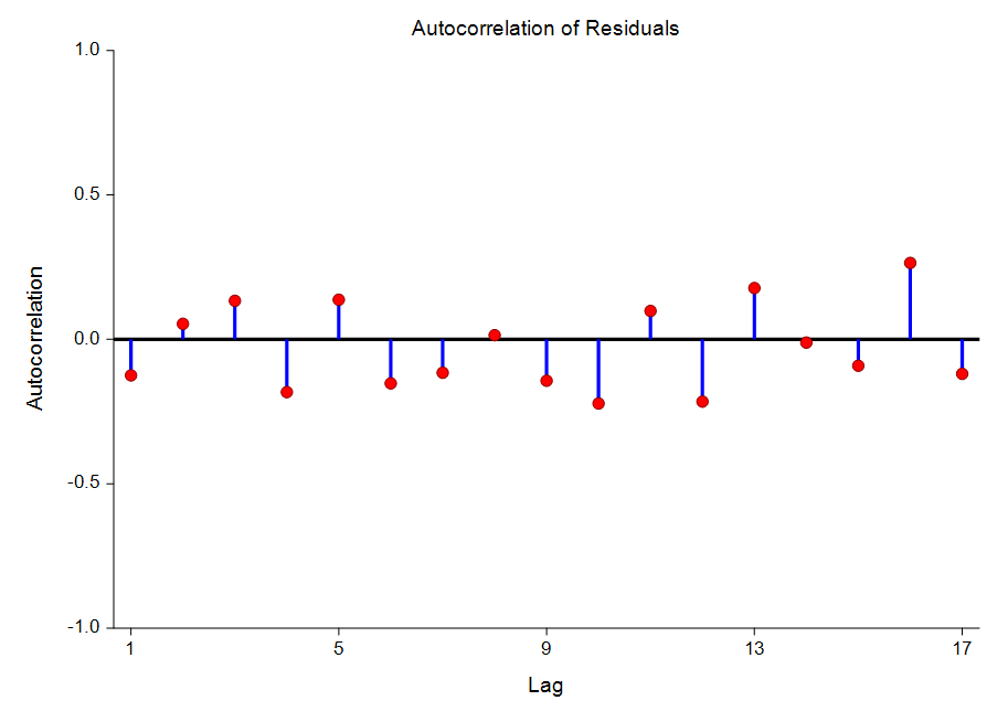
[Documentation PDF]Although the theory behind ARIMA time series models was developed much earlier, the systematic procedure for applying the technique was documented in the landmark book by Box and Jenkins (1976). Since then, ARIMA forecasting and Box-Jenkins forecasting usually refer to the same set of techniques. Box - Jenkins Analysis refers to a systematic method of identifying, fitting, checking, and using integrated autoregressive, moving average (ARIMA) time series models. The method is appropriate for time series of medium to long length (at least 50 observations). A time series is a set of values observed sequentially through time. The series may be denoted by X1, X2, X3, ..., Xt, where t refers to the time period and X refers to the value. If the X’s are exactly determined by a mathematical formula, the series is said to be deterministic. If future values can be described only by their probability distribution, the series is said to be a statistical or stochastic process. A special class of stochastic processes is a stationary stochastic process. A statistical forecasting process is stationary if the probability distribution is the same for all starting values of t. This implies that the mean and variance are constant for all values of t. A series that exhibits a simple trend is not stationary because the values of the series depend on t. A stationary stochastic process is completely defined by its mean, variance, and autocorrelation function. One of the steps in the Box - Jenkins method is to transform a non-stationary series into a stationary one. The stationary assumption allows us to make simple statements about the correlation between two successive values. This correlation is called the autocorrelation of lag k of the series. The autocorrelation function displays the autocorrelation on the vertical axis for successive values of k on the horizontal axis. Since a stationary series is completely specified by its mean, variance, and autocorrelation function, one of the major (and most subjective) tasks in Box-Jenkins analysis is to identify an appropriate model from the sample autocorrelation function. Although the sample autocorrelations contains random fluctuations, for moderate sample sizes they are fairly accurate in signaling the order of the ARIMA model. Further details about this procedure can be obtained by downloading and installing the free trial of the software and going to the help documentation. Some of the available reports in this procedure include the minimization report, the parameter correlation report, the autocorrelation report, the Portmanteau test report, and the forecast report.
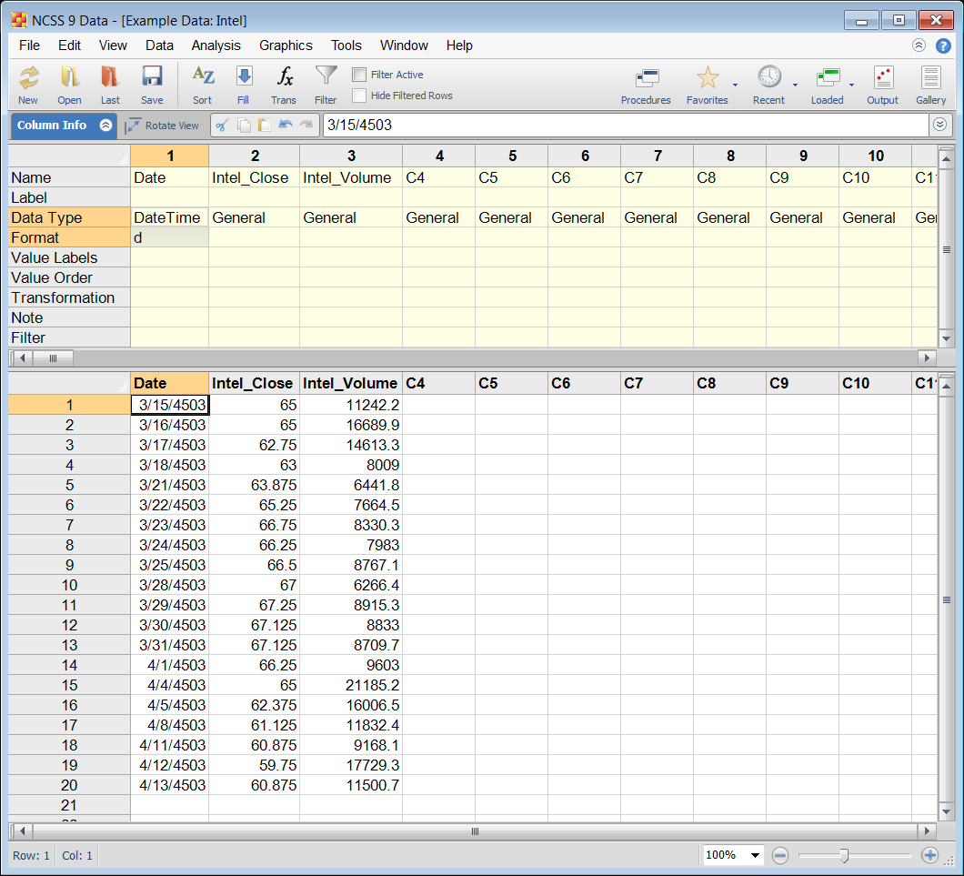
Example Dataset of Time Series Data
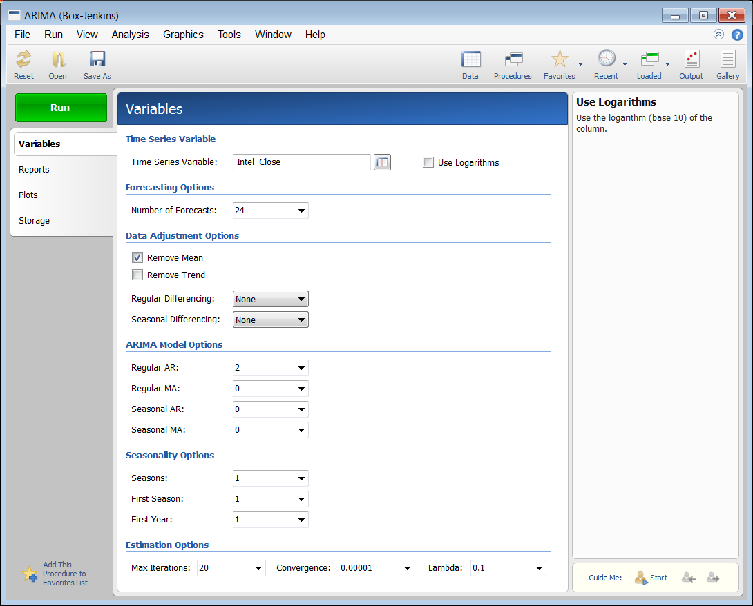
Example Setup of the ARIMA (Box-Jenkins) Procedure
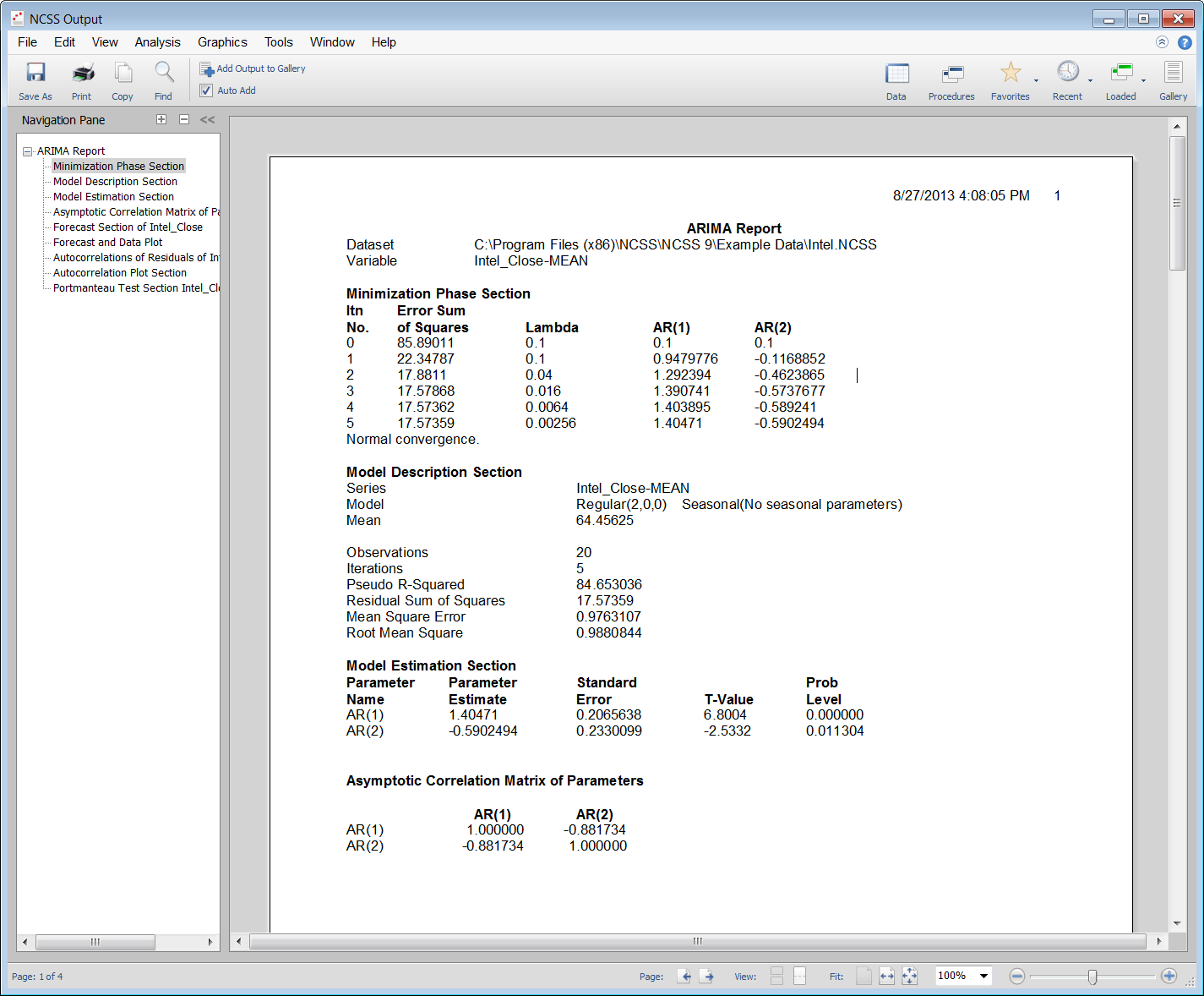
Example Output for the ARIMA (Box-Jenkins) Procedure
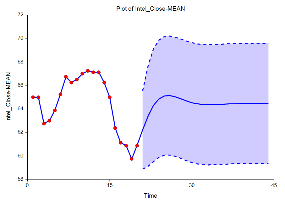
Some Plots from the ARIMA (Box-Jenkins) Procedure
Spectral Analysis
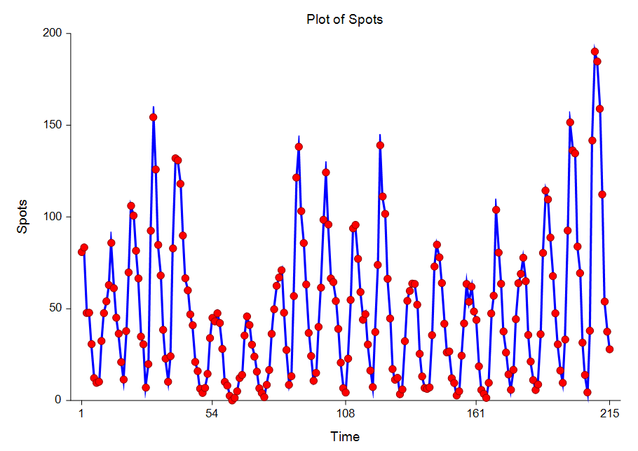
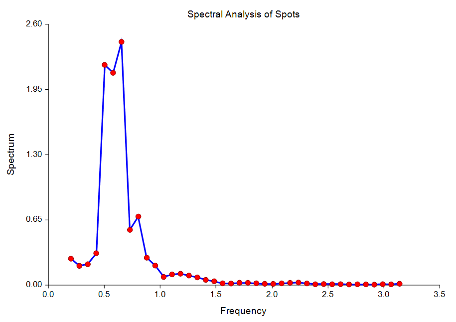
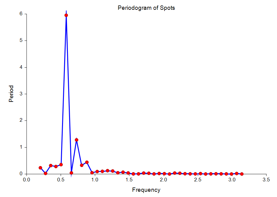
[Documentation PDF]This procedure calculates and displays the periodogram and spectrum of a time series. This is sometimes known as harmonic analysis or the frequency approach to time series analysis. The output also includes a Fourier analysis section.
Some Plots from the Spectral Analysis Procedure
Decomposition Forecasting
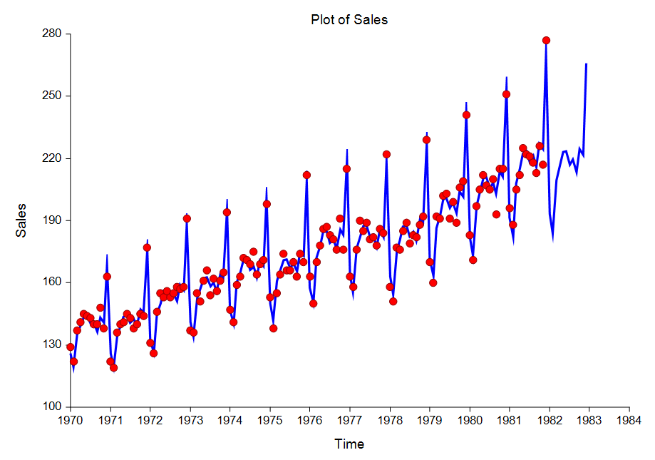
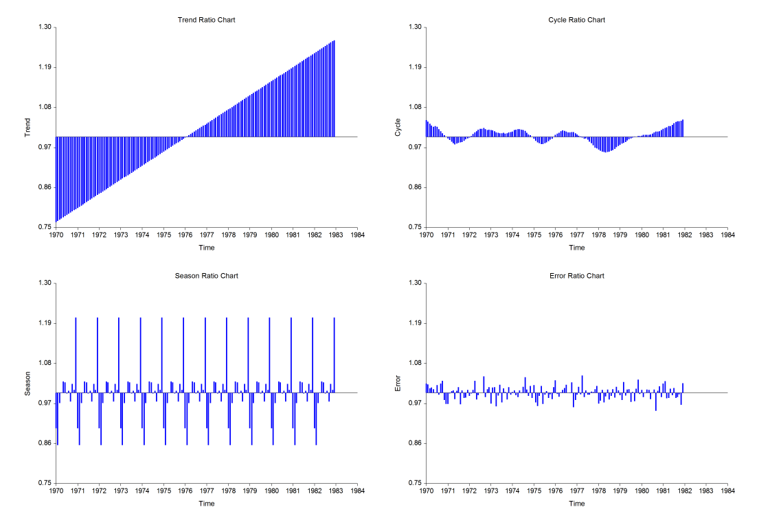
[Documentation PDF]Classical time series decomposition separates a time series into five components: mean, long-range trend, seasonality, cycle, and randomness. The decomposition model is Value = (Mean) x (Trend) x (Seasonality) x (Cycle) x (Random). Note that this model is multiplicative rather than additive. Although additive models are more popular in other areas of statistics, forecasters have found that the multiplicative model fits a wider range of forecasting situations. Decomposition is popular among forecasters because it is easy to understand (and explain to others). While complex ARIMA models are often popular among statisticians, they are not as well accepted among forecasting practitioners. For seasonal (monthly, weekly, or quarterly) data, decomposition methods are often as accurate as the ARIMA methods and they provide additional information about the trend and cycle which may not be available in ARIMA methods. Decomposition has one disadvantage: the cycle component must be input by the forecaster since it is not estimated by the algorithm. You can get around this by ignoring the cycle, or by assuming a constant value. Some forecasters consider this a strength because it allows the forecaster to enter information about the current business cycle into the forecast.
Some Plots from the Decomposition Forecasting Procedure
Exponential Smoothing
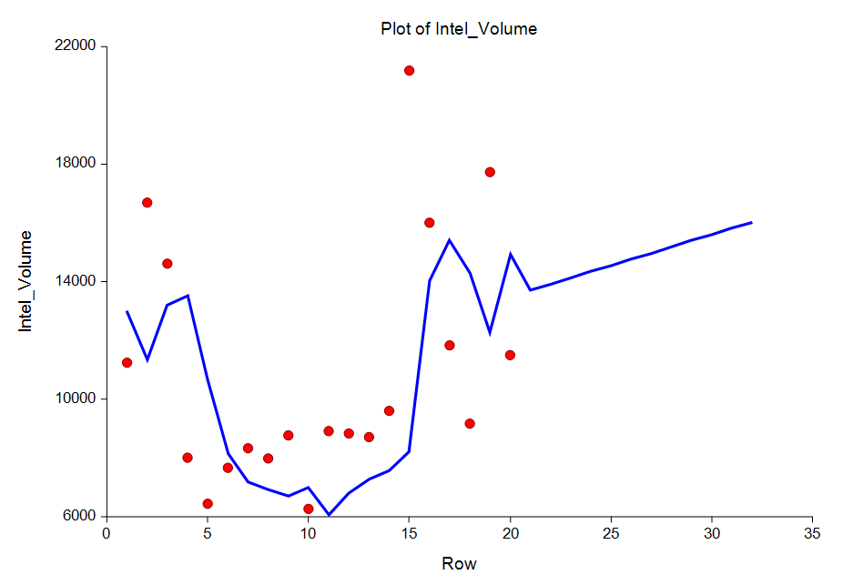
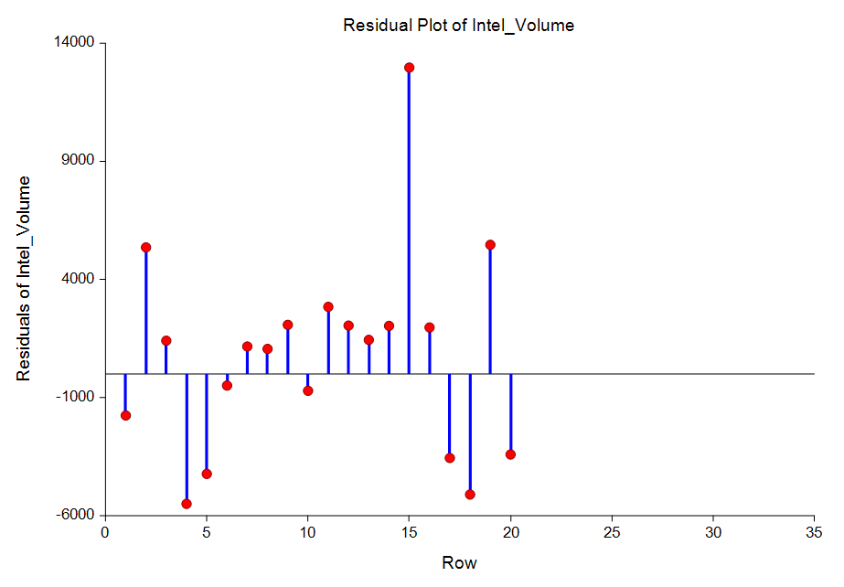
[Documentation PDF for Exponential Smoothing - Horizontal]Exponential smoothing is a technique for making forecasts based on time series data. There are three procedures in NCSS for exponential smoothing:
- Exponential Smoothing - Horizontal
- Exponential Smoothing - Trend
- Exponential Smoothing - Trend / Seasonal
Some Plots from the Exponential Smoothing Procedures
Autocorrelations
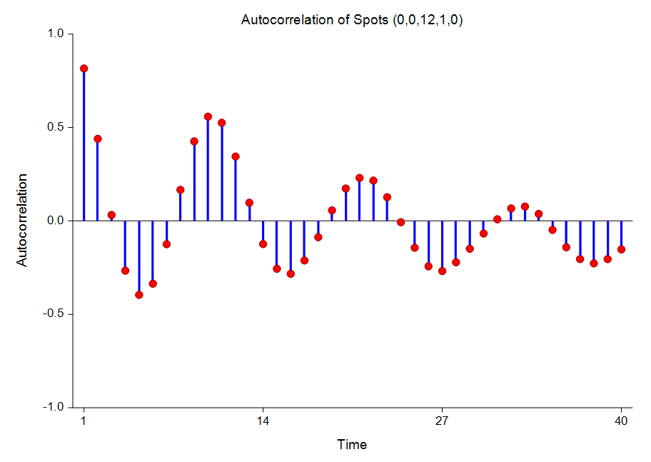
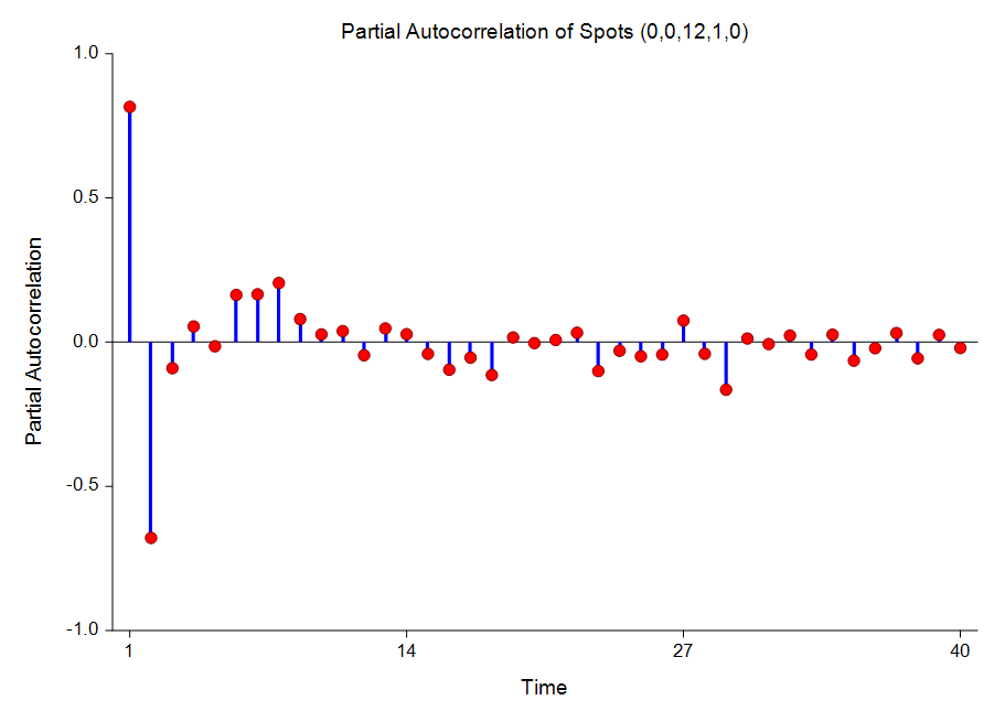
[Documentation PDF]Autocorrelations are used extensively in time series analysis. When plotted, they become the correlogram which is used during the identification phase of the Box-Jenkins method. This procedure provides autocorrelation plots and autocorrelation numeric results, as well as partial autocorrelation plots and numeric results.
Some Plots from the Autocorrelations Procedure
Cross-Correlations
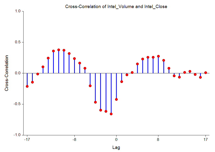
[Documentation PDF]This procedure gives a numeric report of the cross-correlations as well as a plot of the cross-correlations by lag.
A Cross-Correlation Plot from the Cross-Correlations Procedure
Automatic ARMA
[Documentation PDF]The ARIMA (or Box-Jenkins) method is often used to forecast time series of medium (N over 50) to long lengths. It requires the forecaster to be highly trained in selecting the appropriate model. The Automatic ARMA automates the ARIMA forecasting process using a series of algorithms to select the appropriate model. The Automatic ARMA program uses methodology from several authors to find and estimate an appropriate forecasting model. The method may be outlined as follows:
- Using the model selection theory of Pandit and Wu, any deterministic trend is removed from the series.
- A set of models of increasing complexity is fit. These are ARIMA(1,0,0), ARIMA(2,0,1), ARIMA(4,0,3), ARIMA(6,0,5), and so on, increasing both p and q by two at each step. The most complex model tried is specified in the Maximum Order box. The residual sum of squares is calculated for each model and the minimum is noted.
- Using the minimum residual sum of squares as the criterion, the models are again arranged from simplest to most complex. The first model to be within the user-defined percentage of the minimum sum of squares is selected and used.
- Once this model has been determined, one final attempt is made to find a model of smaller order that is within the specified percentage of the minimum. Suppose the previous steps lead to an ARIMA(4,3) model. This step would fit an ARIMA(3,0,2) model and check to see if the residual sum of squares was within the specified percentage. If it was, the ARIMA(3,0,2) model would be used. If not, the ARIMA(4,3) model would be used.
Theoretical ARMA
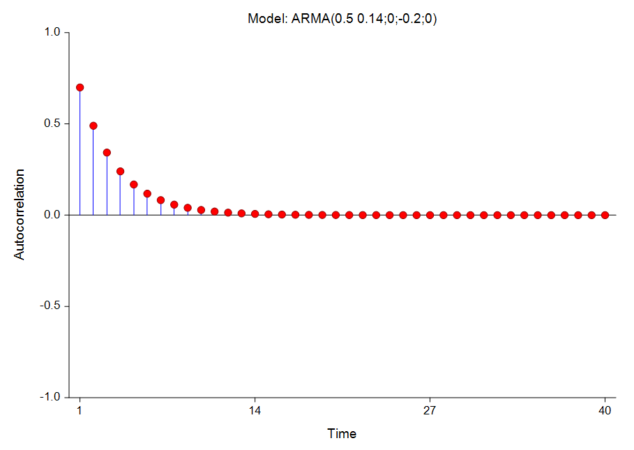
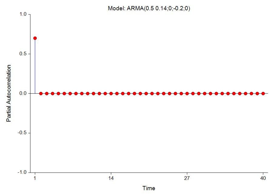
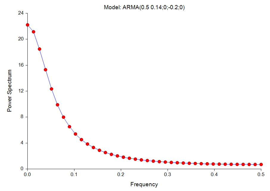
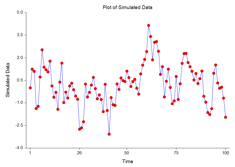
[Documentation PDF]This procedure shows the theoretical characteristics of the autocorrelations, partial autocorrelations, and spectrum of user-specified ARMA models. Unlike the other time series programs, this one does not use data. Instead, it provides a theoretical analysis of various models. It also creates simulated series from these models. We have found this procedure especially useful in training and model evaluation. While you are becoming familiar with the Box-Jenkins method, this program lets you study the characteristics of a large number of models. You will be able to see the sensitivity of the autocorrelation function to changes in the number of, and values of, parameters. You will be able to generate series from known models and see how difficult it is to identify the model from which they came. For use in theoretical model evaluation, this program factors a model written as a polynomial in the backshift operator. This will let you compare several models that each seem adequate, but appear quite different. It will let you study the characteristics of various models in detail. It is useful in model identification, because it will let you generate a catalog of possible autocorrelation patterns from known theoretical models with which you can compare sample autocorrelation functions.
Some Plots from the Theoretical ARMA Procedure
