ROC Curves in NCSS
NCSS contains procedures for single sample ROC curve analysis and for comparing two ROC curves. Use the links below to jump to a ROC Curve topic. To see how these tools can benefit you, we recommend you download and install the free trial of NCSS. Jump to:- Introduction and Discussion
- Other Technical Details
- One ROC Curve and Cutoff Analysis
- Comparing Two ROC Curves - Paired Design
- Comparing Two ROC Curves - Independent Groups Design
Introduction and Discussion
Although ROC curve analysis can be used for a variety of applications across a number of research fields, we will examine ROC curves through the lens of diagnostic testing. In a typical diagnostic test, each unit (e.g., individual or patient) is measured on some scale or given a score with the intent that the measurement or score will be useful in classifying the unit into one of two conditions (e.g., Positive / Negative, Yes / No, Diseased / Non-diseased). Based on a (hopefully large) number of individuals for which the score and condition is known, researchers may use ROC curve analysis to determine the ability of the score to classify or predict the condition. The analysis may also be used to determine the optimal cutoff value (optimal decision threshold). For a given cutoff value, a positive or negative diagnosis is made for each unit by comparing the measurement to the cutoff value. If the measurement is less (or greater, as the case may be) than the cutoff, the predicted condition is negative. Otherwise, the predicted condition is positive. However, the predicted condition doesn’t necessarily match the true condition of the experimental unit (patient). There are four possible outcomes: true positive, true negative, false positive, false negative.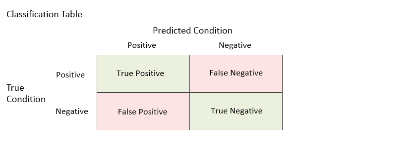 Each unit falls into only one of the four outcomes. When all of the units are assigned to the four outcomes for a given cutoff, a count for each outcome is produced. The four counts are labeled A, B, C, and D in the table below.
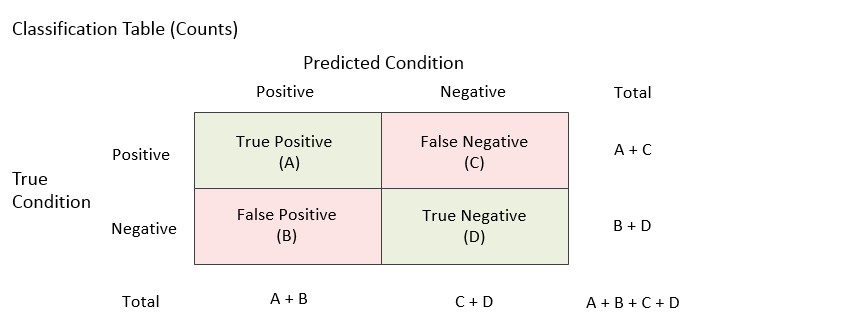 Various rates (proportions) can be used to describe a classification table. Some rates are based on the true condition, some rates are based on the predicted condition, and some rates are based on the whole table. These rates will be described in the following sections.
Rates Assuming a True Condition
The following rates assume one of the two true conditions.True Positive Rate (TPR) or Sensitivity = A / (A + C)
The true positive rate is the proportion of the units with a known positive condition for which the predicted condition is positive. This rate is often called the sensitivity, and constitutes the Y axis on the ROC curve.
True Negative Rate (TNR) or Specificity = D / (B + D)
The true negative rate is the proportion of the units with a known negative condition for which the predicted condition is negative. This rate is often called the specificity. One minus this value constitutes the X axis on the ROC curve.
False Negative Rate (FNR) or Miss Rate = C / (A + C)
The false negative rate is the proportion of the units with a known positive condition for which the predicted condition is negative. This rate is sometimes called the miss rate.
False Positive Rate (FPR) or Fall-out = B / (B + D)
The false positive rate is the proportion of the units with a known negative condition for which the predicted condition is positive. This rate is sometimes called the fall-out, and constitutes the X axis on the ROC curve.
Rates Assuming a Predicted Condition
The following rates assume one of the two predicted conditions.Positive Predictive Value (PPV) or Precision = A / (A + B)
The positive predictive value is the proportion of the units with a predicted positive condition for which the true condition is positive. This rate is sometimes called the precision.
Positive Predictive Value Adjusted for Known Prevalence
When the prevalence (or pre-test probability of a positive condition) is known for the experimental units, an adjusted formula for positive predictive value, based on the known prevalence value, can be used. Using Bayes theorem, adjusted values of PPV are calculated based on known prevalence values as follows:
Negative Predictive Value (NPV) = D / (C + D)
The negative predictive value is the proportion of the units with a predicted negative condition for which the true condition is negative.
Negative Predictive Value Adjusted for Known Prevalence
When the prevalence (or pre-test probability of a positive condition) is known for the experimental units, an adjusted formula for negative predictive value, based on the known prevalence value, can be used. Using Bayes theorem, adjusted values of NPV are calculated based on known prevalence values as follows:
False Omission Rate (FOR) = C / (C + D)
The false omission rate is the proportion of the units with a predicted negative condition for which the true condition is positive.
False Discovery Rate (FDR) = B / (A + B)
The false discovery rate is the proportion of the units with a predicted positive condition for which the true condition is negative.
Whole Table Rates
The following rates are proportions based on all the units.Prevalence = (A + C) / (A + B + C + D)
The prevalence may be estimated from the table if all the units are randomly sampled from the population.
Accuracy or Proportion Correctly Classified = (A + D) / (A + B + C + D)
The accuracy reflects the total proportion of units that are correctly predicted or classified.
Proportion Incorrectly Classified = (B + C) / (A + B + C + D)
The proportion incorrectly classified reflects the total proportion of units that are incorrectly predicted or classified.
Confidence Intervals for Rates (Proportions)
Confidence limits for the above rates are calculated using the exact (Binomial distribution) methods described in the One Proportion chapter of the documentation.Other Diagnostic Accuracy Indices
Over the past several decades, a number of table summary indices have been considered, above those described above. Those available in NCSS are described below.Youden Index
Conceptually, the Youden index is the vertical distance between the 45 degree line and the point on the ROC curve. The formula for the Youden index is Higher values of the Youden index are better than lower values.
Sensitivity + Specificity
The addition of the sensitivity and the specificity gives essentially the same information as the Youden index, but may be slightly more intuitive for interpretation. Higher values of sensitivity plus specificity are better than lower values.Distance to Corner
The distance to the top-left corner of the ROC curve for each cutoff value is given by Lower distances to the corner are better than higher distances.
Positive Likelihood Ratio (LR+) = TPR / FPR
The positive likelihood ratio is the ratio of the true positive rate (sensitivity) to the false positive rate (1 – specificity). This likelihood ratio statistic measures the value of the test for increasing certainty about a positive diagnosis.
Negative Likelihood Ratio (LR-) = FNR / TNR
The negative likelihood ratio is the ratio of the false negative rate to the true negative rate (specificity).
Diagnostic Odds Ratio (DOR) = LR+ / LR-
The diagnostic odds ratio is the ratio of the positive likelihood ratio to the negative likelihood ratio.
Cost
A cost approach is sometimes used when seeking to determine the optimal cutoff value. This approach is based on an analysis of the costs of the four possible outcomes of a diagnostic test: true positive (TP), true negative (TN), false positive (FP), and false negative (FN). If the cost of each of these outcomes is known. The average overall cost C of performing a test at a given cutoff is given by In order to make these cost calculations, known prevalence and cost values (or cost ratio) must be supplied.
ROC Curves
Each of the rates above are calculated for a given table, based on a single cutoff value. A receiver operating characteristic (ROC) curve plots the true positive rate (sensitivity) against the false positive rate (1 – specificity) for all possible cutoff values. Two types of ROC curves can be generated in NCSS: the empirical ROC curve and the binormal ROC curve.Empirical ROC Curve
The empirical ROC curve is the more common version of the ROC curve. The empirical ROC curve is a plot of the true positive rate versus the false positive rate for all possible cut-off values.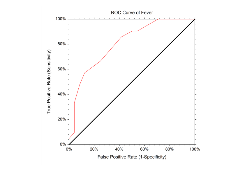 That is, each point on the ROC curve represents a different cutoff value. The points are connected to form the curve. Cutoff values that result in low false-positive rates tend to result low true-positive rates as well. As the true-positive rate increases, the false positive rate increases. The better the diagnostic test, the more quickly the true positive rate nears 1 (or 100%). A near-perfect diagnostic test would have an ROC curve that is almost vertical from (0,0) to (0,1) and then horizontal to (1,1). The diagonal line serves as a reference line since it is the ROC curve of a diagnostic test that randomly classifies the condition.
Binormal ROC Curve
The Binormal ROC curve is based on the assumption that the diagnostic test scores corresponding to the positive condition and the scores corresponding to the negative condition can each be represented by a Normal distribution. To estimate the Binormal ROC curve, the sample mean and sample standard deviation are estimated from the known positive group, and again for the known negative group. These sample means and sample standard deviations are used to specify two Normal distributions. The Binormal ROC curve is then generated from the two Normal distributions. When the two Normal distributions closely overlap, the Binormal ROC curve is closer to the 45 degree diagonal line. When the two Normal distributions overlap only in the tails, the Binormal ROC curve has a much greater distance from the 45 degree diagonal line.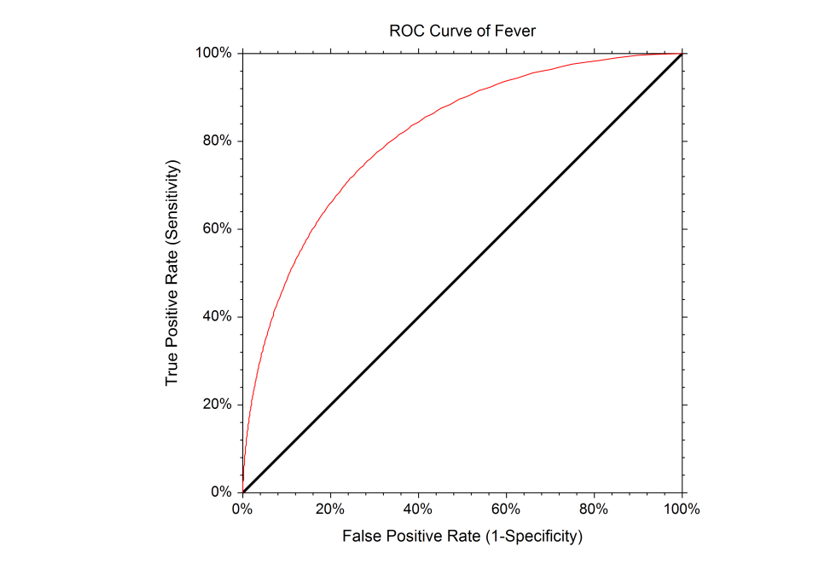 It is recommended that researchers identify whether the scores for the positive and negative groups need to be transformed to more closely follow the Normal distribution before using the Binormal ROC Curve methods.
Area under the ROC Curve (AUC)
The area under an ROC curve (AUC) is a popular measure of the accuracy of a diagnostic test. In general higher AUC values indicate better test performance. The possible values of AUC range from 0.5 (no diagnostic ability) to 1.0 (perfect diagnostic ability). The AUC has a physical interpretation. The AUC is the probability that the criterion value of an individual drawn at random from the population of those with a positive condition is larger than the criterion value of another individual drawn at random from the population of those where the condition is negative. Another interpretation of AUC is the average true positive rate (average sensitivity) across all possible false positive rates. Two methods are commonly used to estimate the AUC. One method is the empirical (nonparametric) method. This method has become popular because it does not make the strong normality assumptions that the Binormal method makes. The other method is the Binormal method. This method results in a smooth ROC curve from which the complete (and partial) AUC may be calculated.Other Technical Details
The discussion above gives a general overview of many of the diagnostic test summary statistics. If you would like to examine the formulas and technical details relating to a specific NCSS procedure, click on the corresponding '[Documentation PDF]' link under each heading to load the complete procedure documentation. There you will find formulas, references, discussions, and examples or tutorials describing the procedure in detail.One ROC Curve and Cutoff Analysis
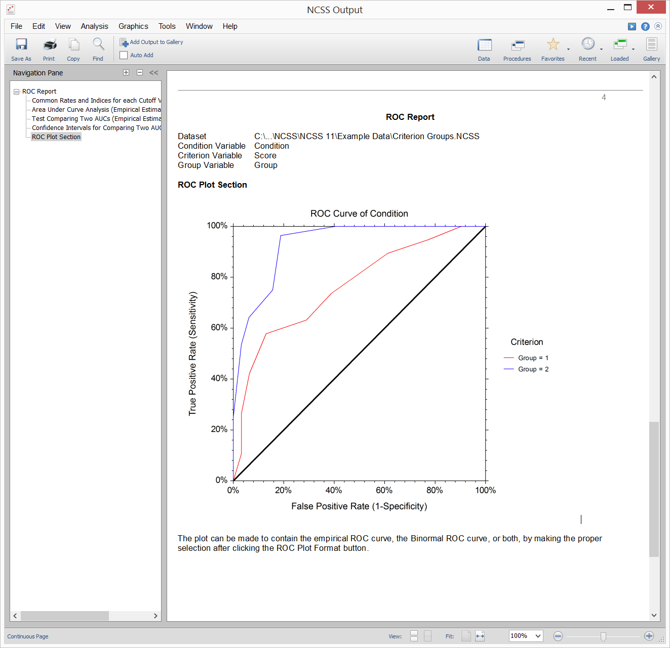
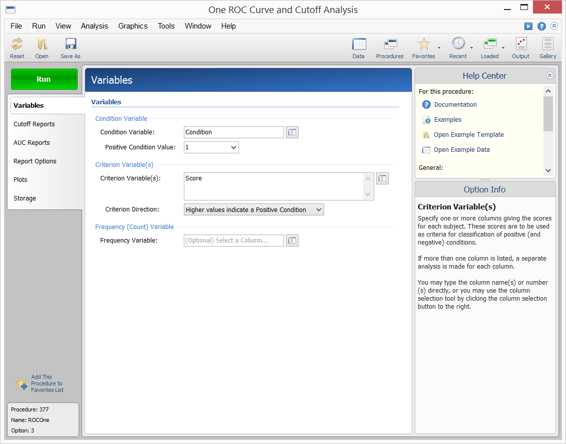
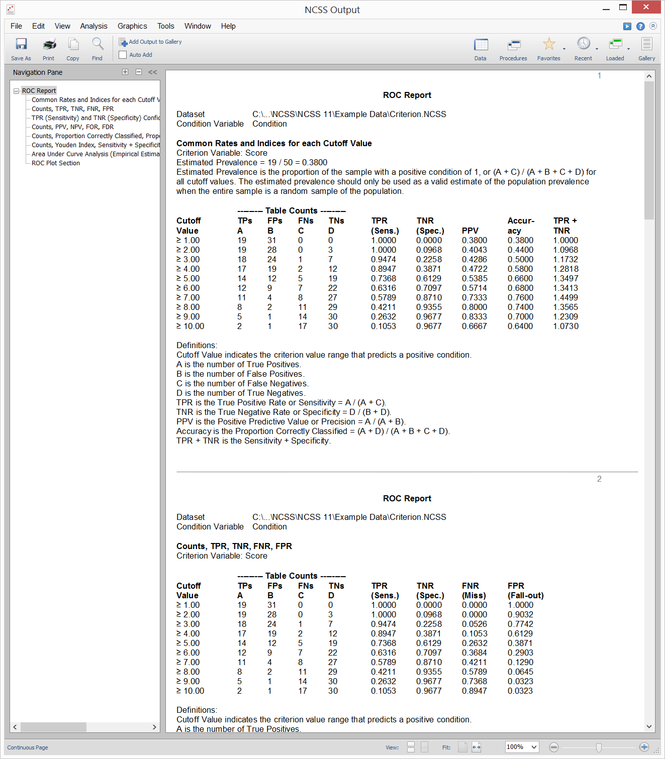
[Documentation PDF]The One ROC Curve and Cutoff Analysis procedure generates empirical (nonparametric) and Binormal ROC curves. It also gives the area under the ROC curve (AUC), the corresponding confidence interval of AUC, and a statistical test to determine if AUC is greater than a specified value. Summary measures for a desired (user-specified) list of cutoff values are also available. Some of these measures include sensitivity, specificity, proportion correctly specified, table counts, positive predictive value, cost analysis, likelihood ratios, and the Youden index. These measure are often used to determine the optimal cutoff value (optimal decision threshold).
ROC Curve Analysis Example Dataset

Example Setup of the One ROC Curve and Cutoff Analysis Procedure
Example Output for the One ROC Curve and Cutoff Analysis Procedure
Comparing Two ROC Curves - Paired Design
[Documentation PDF]This procedure is used to compare two ROC curves for the paired sample case wherein each subject has a known condition value and test values (or scores) from two diagnostic tests. The test values are paired because they are measured on the same subject. In addition to producing a wide range of cutoff value summary rates for each criterion, this procedure produces difference tests, equivalence tests, non-inferiority tests, and confidence intervals for the difference in the area under the ROC curve. This procedure includes analyses for both empirical (nonparametric) and Binormal ROC curve estimation.
Comparing Two ROC Curves - Independent Groups Design
[Documentation PDF]This procedure is used to compare two ROC curves generated from data from two independent groups. In addition to producing a wide range of cutoff value summary rates for each group, this procedure produces difference tests, equivalence tests, non-inferiority tests, and confidence intervals for the difference in the area under the ROC curve. This procedure includes analyses for both empirical (nonparametric) and Binormal ROC curve estimation.
