Quality Control in NCSS

NCSS contains several tools and charts for analyzing quality control, including X-bar, R, s, P, NP, C, U, EWMA, CUSUM, Individuals, Moving Range, Pareto, and Levey-Jennings charts. Each procedure is easy to use and is validated for accuracy. Use the links below to jump to a quality control topic. To see how these tools can benefit you, we recommend you download and install the free trial of NCSS. Jump to:

Introduction
Technical Details
X-bar, R, s, CUSUM, EWMA, Moving Average, Individuals, and Moving Range Charts
P, NP, C, and U Charts
Levey-Jennings Charts
Pareto Charts
R & R Study
Capability Analysis
Lag Plots
Box-Cox Transformation
Acceptance Sampling for Attributes
Operating Characteristic Curves for Acceptance Sampling for Attributes

Introduction

The quality control procedures in NCSS are visual and numeric tools used to monitor whether a process is in control by examining whether measurement summaries stay within the specified precision limits.

Technical Details

This page provides a general overview of the tools that are available in NCSS for statistical quality control. If you would like to examine the formulas and technical details relating to a specific NCSS procedure, click on the corresponding '[Documentation PDF]' link under each heading to load the complete procedure documentation. There you will find formulas, references, discussions, and examples or tutorials describing the procedure in detail.

X-bar, R, s, CUSUM, EWMA, Moving Average, Individuals, and Moving Range Charts

[Documentation PDF (X-bar and R)]

[Documentation PDF (CUSUM)]

[Documentation PDF (EWMA)]

[Documentation PDF (Individuals and Moving Range)]

These procedures generate various control charts useful for monitoring the average and variability of a process. The X-bar, EWMA, Moving Average, Individuals, Range, Standard deviation, Moving Range, and CUSUM charts are available. Capability analysis and various reports are also available.

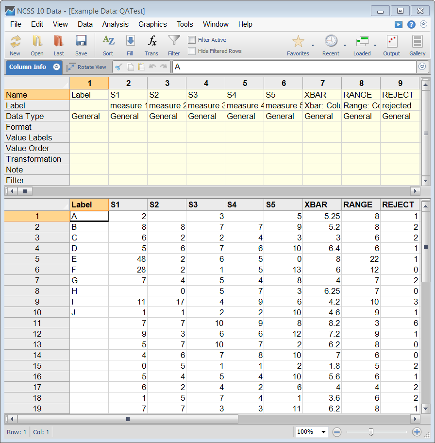
Example Dataset of X-bar and R Chart Data

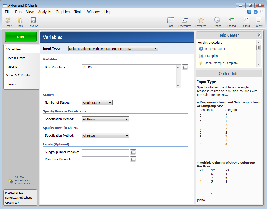
Example Setup of the X-bar and R Chart Procedure

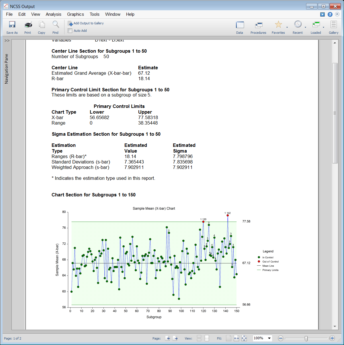
Example Output for the X-bar and R Chart Procedure

P, NP, C, and U Charts

[Documentation PDF (P)]

[Documentation PDF (NP)]

[Documentation PDF (C)]

[Documentation PDF (U)]

These charts are useful for displaying count data such as the number of defectives or the number of defects on a certain item. Here is a brief description of each of these four charts:

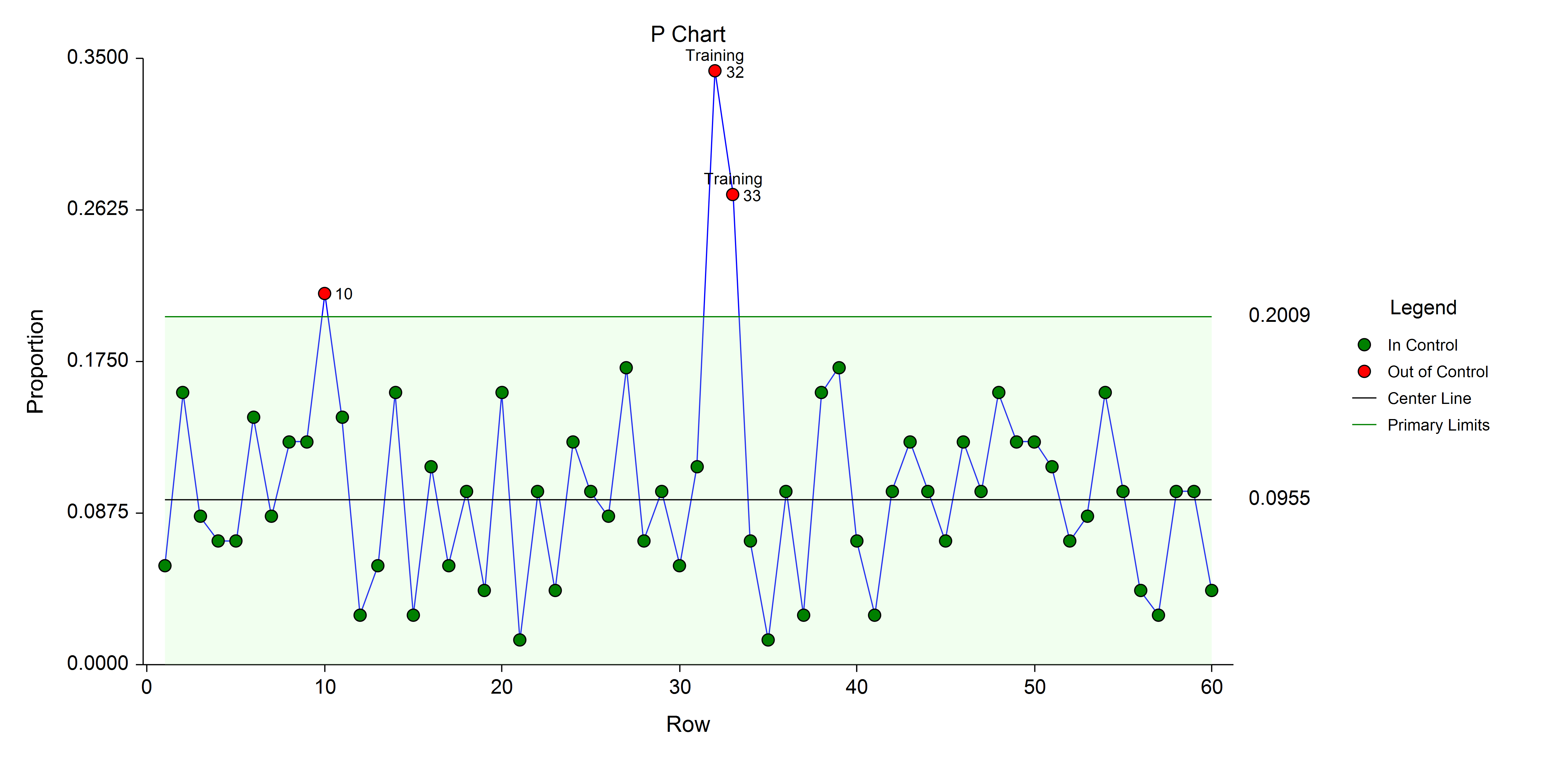
P Chart: The charted value is the fraction defective in a sample of n items. Probability calculations are based on the binomial distribution.
NP Chart: The charted value is the number defective in a sample of n items per time period. The chart is very confusing if the sample size, n, is not constant from period to period. Probability calculations are based on the binomial distribution.
C Chart: The charted value is the number of defects on an item. Probability calculations are based on the Poisson distribution.
U Chart: The charted value is the average number of defects on n items. Probability calculations are based on the Poisson distribution.

An Example P Chart

Levey-Jennings Charts

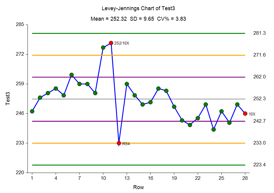
[Documentation PDF]

This procedure generates Levey-Jennings control charts on single variables. It finds out-of-control points using the Westgard rules. The Levey-Jennings control chart is a special case of the common Shewart X-bar chart in which there is only a single stream of data and sigma is estimated using the standard deviation of those data.

An Example Levey-Jennings Control Chart from the Levey-Jennings Charts Procedure

Pareto Charts

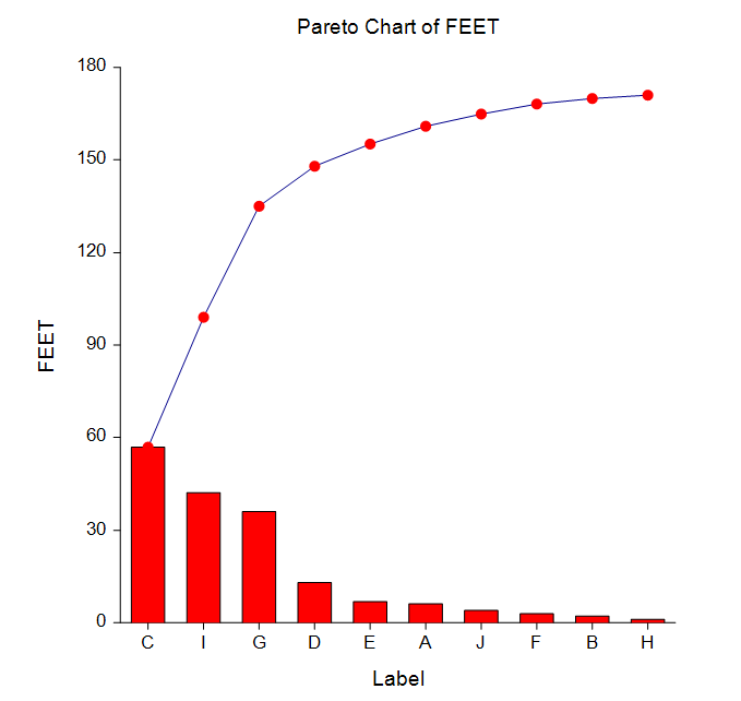
[Documentation PDF]

An Italian economist, Vilfredo Pareto (1848-1923), noticed a great inequality in the distribution of wealth. A few people owned most of the wealth. J. M. Juran found that this same phenomenon of the “vital few and the trivial many” applied to many areas of SPC. He is credited with coining the terms “Pareto chart” and “Pareto analysis” to represent this phenomenon. In quality control, Pareto analysis refers to the tendency for the bulk of the quality problems to be due to a few of the possible sources. Hence, by isolating and correcting the major problem areas, you obtain the greatest increase in quality. The Pareto chart is a graphic display that emphasizes the Pareto principle using a bar graph in which the bars are arranged in decreasing magnitude. NCSS provides two Pareto chart styles as well as a numerical report.

An Example Pareto Chart from the Pareto Charts Procedure

R & R Study

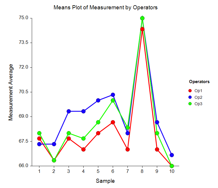
[Documentation PDF]

A repeatability and reproducibility (R & R) study (sometimes called a gauge study) is conducted to determine if a particular measurement procedure is adequate. If the measurement variation is small relative to the actual process variation, the measurement procedure is adequate. If it is not, the measurement procedure must be improved before it can satisfactorily monitor the process. R & R studies separate process variation into the portion due to the measurement procedure and the portion due to the production process itself. The measurement variation is further divided into that due to the appraiser (reproducibility) and that due to the measuring device (repeatability). It is important to emphasize that an R & R study is concerned with the precision of the measurement process. Data for R & R studies should come from experiments specially designed for that purpose. Several booklets are available that discuss R & R studies in detail. We recommend Barrentine (1991) and AIAG (1995). Although both of these concentrate on the “control chart” approach, they mention the analysis of variance approach—which we use here. The AIAG booklet states that the control chart approach is to be used only when software to analyze your data with the analysis of variance approach is not available. Output options available in this procedure include an EMS report, ANOVA report, Variance report, Process Variation and R & R report, Tolerance R & R report, R & R Indices report, and a Means report.

One of Several Plots Available in the R & R Study Procedure

Capability Analysis

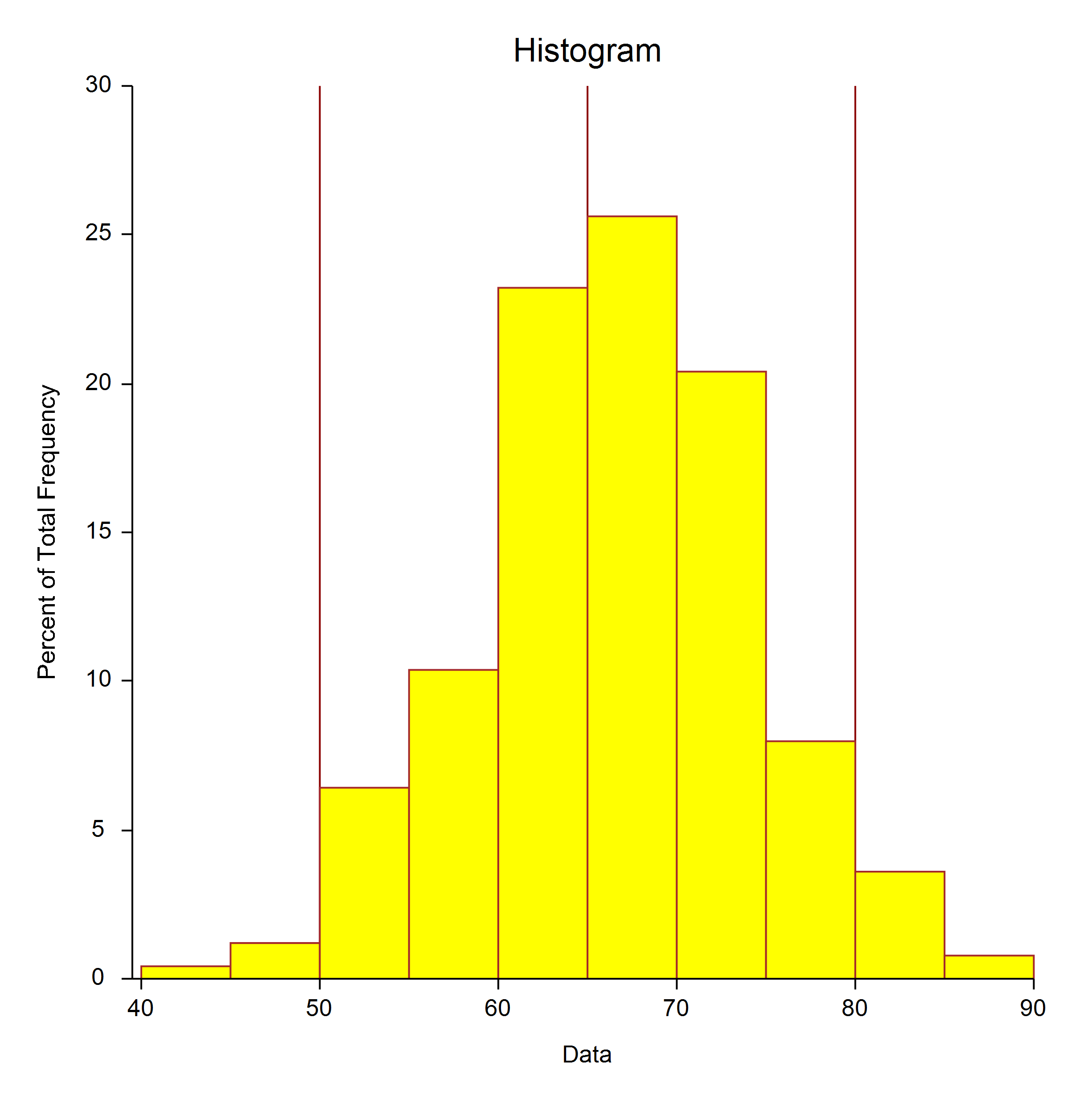
[Documentation PDF]

This procedure summarizes the performance of a process based on user-specified specification limits. The observed performance as well as the performance relative to the Normal distribution are output. Process capability ratios such as Cp and Cpk are produced. Cpm and Cpkm may also be generated if a specification target is entered. A capability histogram with specification limit lines may also be produced in this procedure. Normality Tests are also given in this procedure. Subgroup data or individual values may be used.

An Example Capability Histogram from the Capability Analysis Procedure

Lag Plots

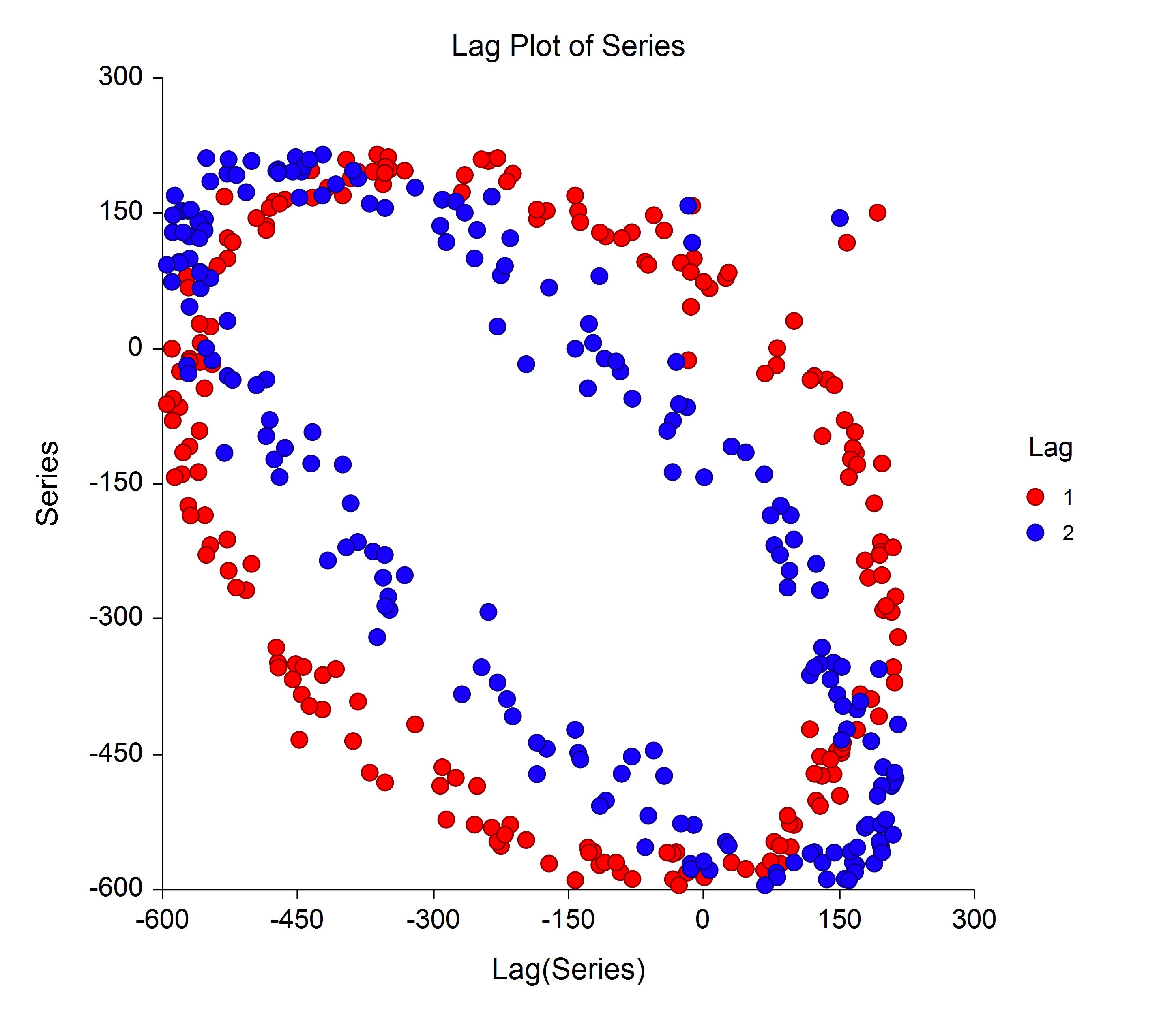
[Documentation PDF]

A lag plot is used to help evaluate whether the values in a dataset or time series are random. If the data are random, the lag plot will exhibit no identifiable pattern. If the data are not random, the lag plot will demonstrate a clearly identifiable pattern. The type of pattern can aid the user in identifying the non-random structure in the data. Lag plots can also help to identify outliers. This procedure will generate all lag plots up to a user-specified maximum lag k in a single run.

An Example Lag Plot from the Lag Plots Procedure

Box-Cox Transformation

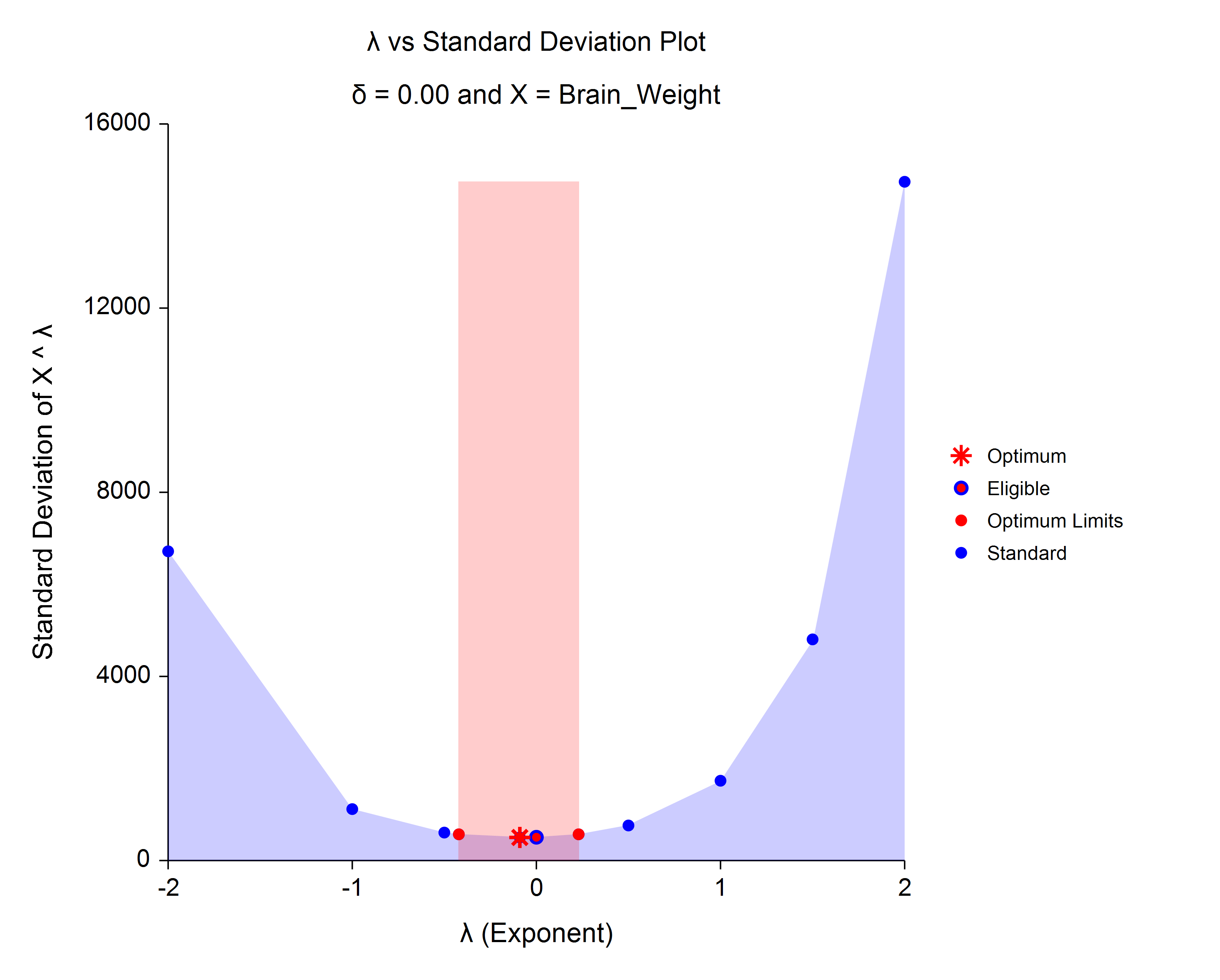
[Documentation PDF]

This procedure finds the appropriate Box-Cox power transformation for a single set of data. It is used to modify the distributional shape of a set of data to be more normally distributed so that tests and confidence limits that require normality can be appropriately used.

An Example Box-Cox Lambda Plot from the Box-Cox Transformation Procedure

Acceptance Sampling for Attributes

[Documentation PDF]

The Acceptance Sampling for Attributes procedure is used to determine the number of items to be sampled from a lot to determine whether to accept or reject the lot. The number of items in the sample depend upon a number of parameters, including the lot size, the acceptable quality level (AQL), the desired producer’s risk, the limiting quality level (LQL, sometimes called the rejectable quality level or lot tolerance percent/proportion defective), and the desired consumer’s risk. This procedure permits the user to enter multiple values of any of these parameters to determine the sensitivity of the sample size to that parameter. When multiple values are entered for a parameter, a sample size curve is also produced. The cutoff value of acceptance, or acceptance number, is also given as part of the output. In this procedure, the lot size can be assumed to be infinite (or continuous) and use the binomial distribution for calculations, or the lot can have a fixed size, whereupon the calculations are based on the hypergeometric distribution.

Operating Characteristic Curves for Acceptance Sampling for Attributes

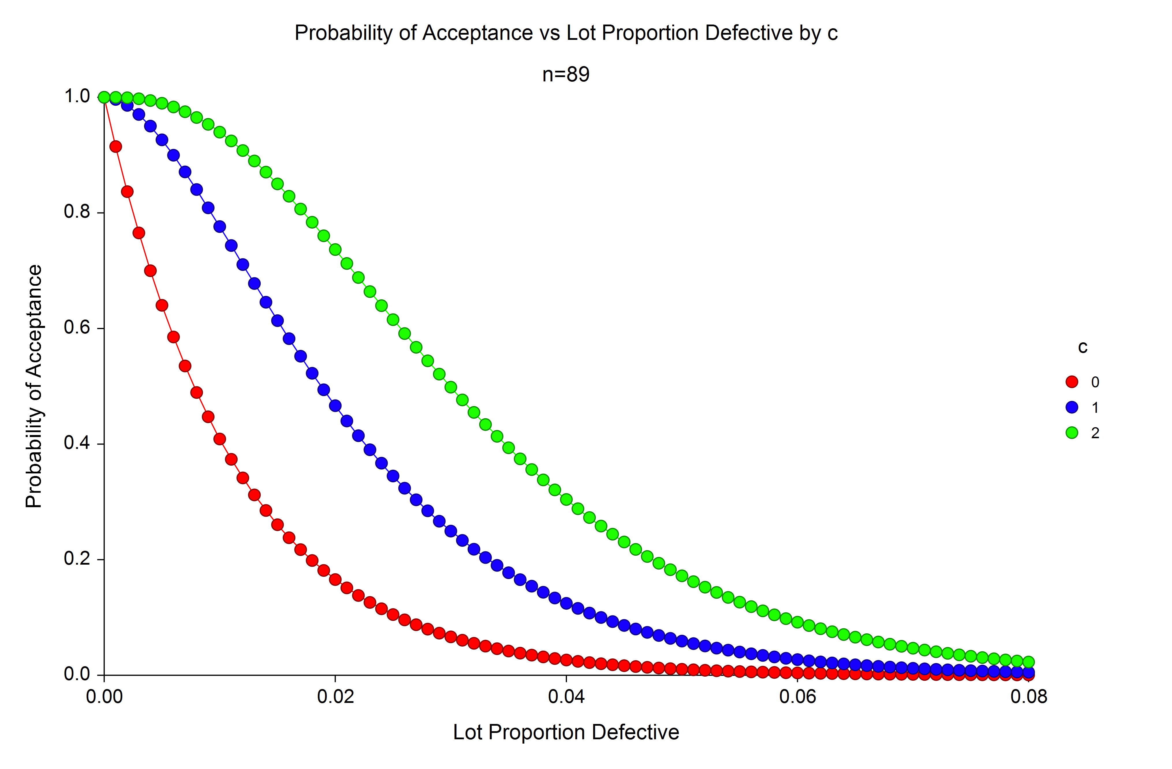
[Documentation PDF]

The Operating Characteristic Curves for Acceptance Sampling for Attributes procedure is a companion procedure to the procedure Acceptance Sampling for Attributes. This procedure is used view graphically the probability of lot acceptance versus the lot proportion defective for a given sample size and acceptance number. Plots with multiple curves for multiple sample sizes or multiple acceptance numbers may be generated using this procedure. In this procedure, the lot size can be assumed to be infinite (or continuous) and use the binomial distribution for calculations, or the lot can have a fixed size, whereupon the calculations are based on the hypergeometric distribution.