Description:
In this session, we will discuss several features that are common to most of the plot format windows in NCSS. These features are saving and opening plot settings files, plot extras, background colors and sizes, the painting order, the example data for previewing plots, and editing plots with your actual data.
We will use the scatter plot format window as an example representing most of the NCSS plots.
More than half of the NCSS procedures have associated plots. In these procedures, plot format windows are accessed by clicking the large plot format buttons.
All the aspects of a plot format can be saved to any folder location by going to the file menu and saving the plot settings file. This settings file can be loaded from any format window of the same type. So if I save my scatter plot settings file while using the scatter plot procedure, I can load those same settings for any of the scatter plots used in the linear regression and correlation procedure. The reset button of the File menu can be used to return all the plot format options to their default values.
It is often useful to add a line, symbol, or note to a specified location on the plot. To do this, go to the extras tab and select the appropriate sub-tab. Here we will use the example of adding a note to the center of the graph.
First we check the box next to the note. The text and the format of the text are easily specified. The default location for the note is the bottom left corner of the interior of the graph. To move the note to the center of the graph, we change the location to 50, 50, based on the axis maximums of 100. The note can then be shifted by individual pixels to the exact desired location.
The background tab is used to specify the background colors, the size of the interior of the plot, and the plot margin sizes. The background fill covers the area of the entire plot. If you wish to have the interior fill hidden to show the background fill, simply uncheck the interior fill checkbox.
The size of the interior rectangle is specified by the width and height of the interior data area. One use for increasing the interior size is to emphasize the interior of the plot. Additional space can be added to the exterior of the overall plot by increasing the margins on this tab.
The painting order of the objects of the graph becomes important when there are objects on the graph that overlap. Objects that are painted last on the plot show up at the front of the plot. To move an object in front of another, select the object and click the down button. Or, to move it to the front of all objects, click the Last button. For example, if we wish to move the regression lines on the plot in front of the plot symbols, we could do so by selecting the Linear Regression Line and clicking the Last button.
When a plot format button is pressed from a procedure, the data from the columns of the data window is not yet a part of the plot. The Example Data tab allows you to specify some general constraints on the example data used to produce the preview plot. The settings for this tab can be used to control the number of groups displayed or the data limits of the values. Each plot will have different example data parameters corresponding to that plot.
If you wish the change the plot format with your actual data integrated into the plot, you can check the box next to the upper right corner of the plot format button. When the procedure is run, the procedure will pause when that graph is created and the plot format window will open with the integrated data as part of the graph. When you click the OK button on the Plot Format window, the changes will take effect on the plot that is produced in the output. Furthermore, if you go back to the procedure window and click the format button, those changes will still be there.
This concludes our discussion of some of the features that are common to most plots.