Regression Analysis in NCSS

NCSS software has a full array of powerful software tools for regression analysis. Below is a list of the regression procedures available in NCSS. You can jump to a description of a particular type of regression analysis in NCSS by clicking on one of the links below. To see how these tools can benefit you, we recommend you download and install the free trial of NCSS. Jump to:

• Introduction
• Technical Details
• 
  
• Simple Linear Regression
• Linear Regression and Correlation
• Box-Cox Transformation for Simple Linear Regression
• Robust Linear Regression (Passing-Bablok Median-Slope)
• 
  
• Multiple Regression
• Multiple Regression
• Principal Components Regression
• Response Surface Regression
• Ridge Regression
• Robust Regression
• 
  
• Logistic Regression
• Logistic Regression
• Conditional Logistic Regression
• 
  
• Nonlinear Regression
• Nonlinear Regression
• Curve Fitting
• 
  
• Regression for Method Comparison
• Deming Regression
• Passing-Bablok Regression
• 
  
• Regression with Survival or Reliability Data
• Cox (Proportional Hazards) Regression
• Parametric Survival (Weibull) Regression
• 
  
• Regression with Count Data
• Poisson Regression
• Zero-Inflated Poisson Regression
• Negative Binomial Regression
• Zero-Inflated Negative Binomial Regression
• Geometric Regression
• 
  
• Regression with Time Series Data
• Multiple Regression with Serial Correlation
• Harmonic Regression
• 
  
• Regression with Nondetects Data
• Nondetects-Data Regression
• 
  
• Two-Stage Least Squares
• Two-Stage Least Squares
• 
  
• Subset Selection
• All Possible Regressions
• Stepwise Regression
• Subset Selection in Multiple Regression
• Subset Selection in Other Regression Procedures
• Subset Selection in Multivariate Y Multiple Regression

Introduction

Regression analysis refers to a group of techniques for studying the relationships among two or more variables based on a sample. NCSS makes it easy to run either a simple linear regression analysis or a complex multiple regression analysis, and for a variety of response types. NCSS has modern graphical and numeric tools for studying residuals, multicollinearity, goodness-of-fit, model estimation, regression diagnostics, subset selection, analysis of variance, and many other aspects that are specific to type of regression being performed.

Technical Details

This page is designed to give a general overview of the capabilities of the NCSS software for regression analysis. If you would like to examine the formulas and technical details relating to a specific NCSS procedure, click on the corresponding '[Documentation PDF]' link under each heading to load the complete procedure documentation. There you will find formulas, references, discussions, and examples or tutorials describing the procedure in detail.

Simple Linear Regression

[Documentation PDF]

Simple Linear Regression refers to the case of linear regression where there is only one X (explanatory variable) and one continuous Y (dependent variable) in the model. Simple linear regression fits a straight line to a set of data points. The simple linear regression model equation is of the form

Y = ?₀ + ?₁X.

NCSS includes three procedures related to simple linear regression:

• 1. Linear Regression and Correlation
• 2. Box-Cox Transformation for Simple Linear Regression
• 3. Robust Linear Regression (Passing-Bablok Median-Slope)

Linear Regression and Correlation

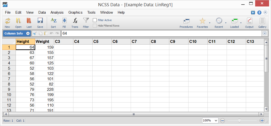
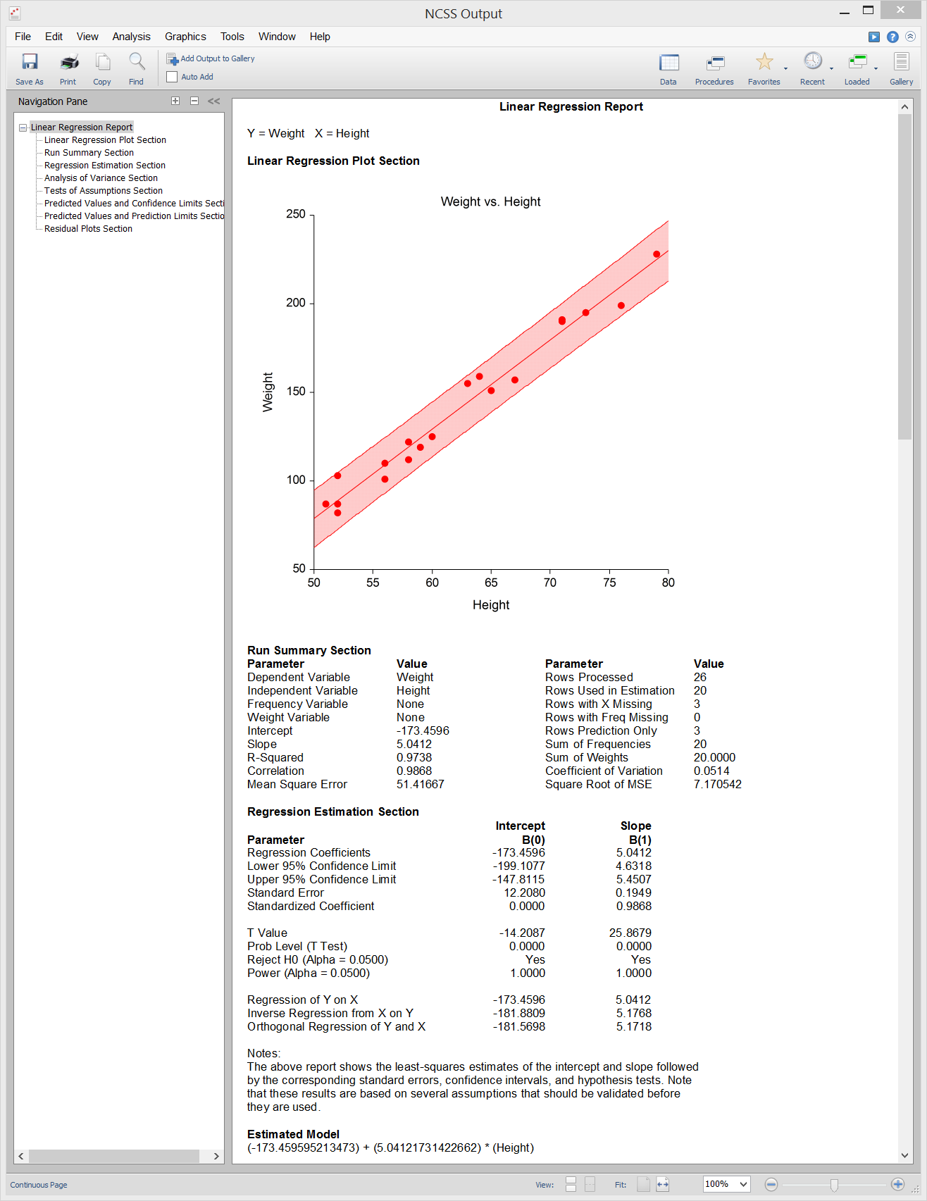
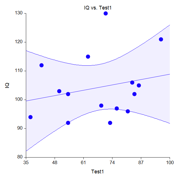
Because a large proportion of regression analyses involve only one independent (X, explanatory) variable, an individual procedure is dedicated to this specific scenario in NCSS. Statistical reports available in this procedure include data and model summaries, correlation and R-Squared analysis, summary matrices, analysis of variance reports, assumptions tests for residuals (do the residuals follow a normal distribution? is the residual variance constant?), a test of lack of linear fit, evaluation of serial correlation through the Durbin-Watson test and serial correlations values, PRESS statistics, predicted values with confidence and prediction limits, outlier detection charts, residual diagnostics, influence detection, leave one row out analysis, predicted values, simultaneous confidence bands, inverse prediction, and more.

Example Linear Regression Plot

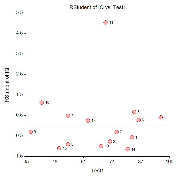
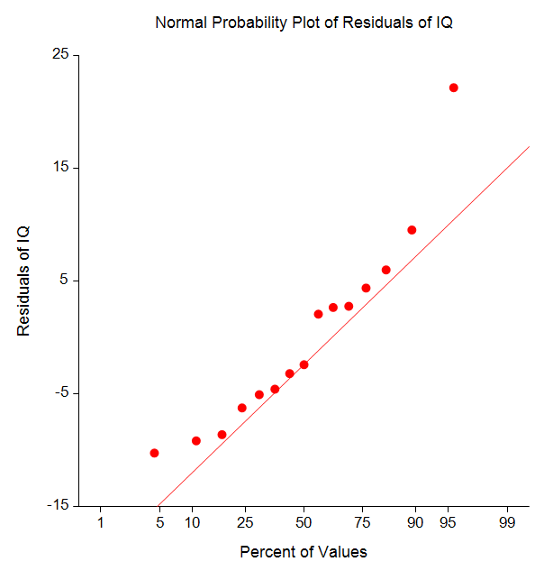
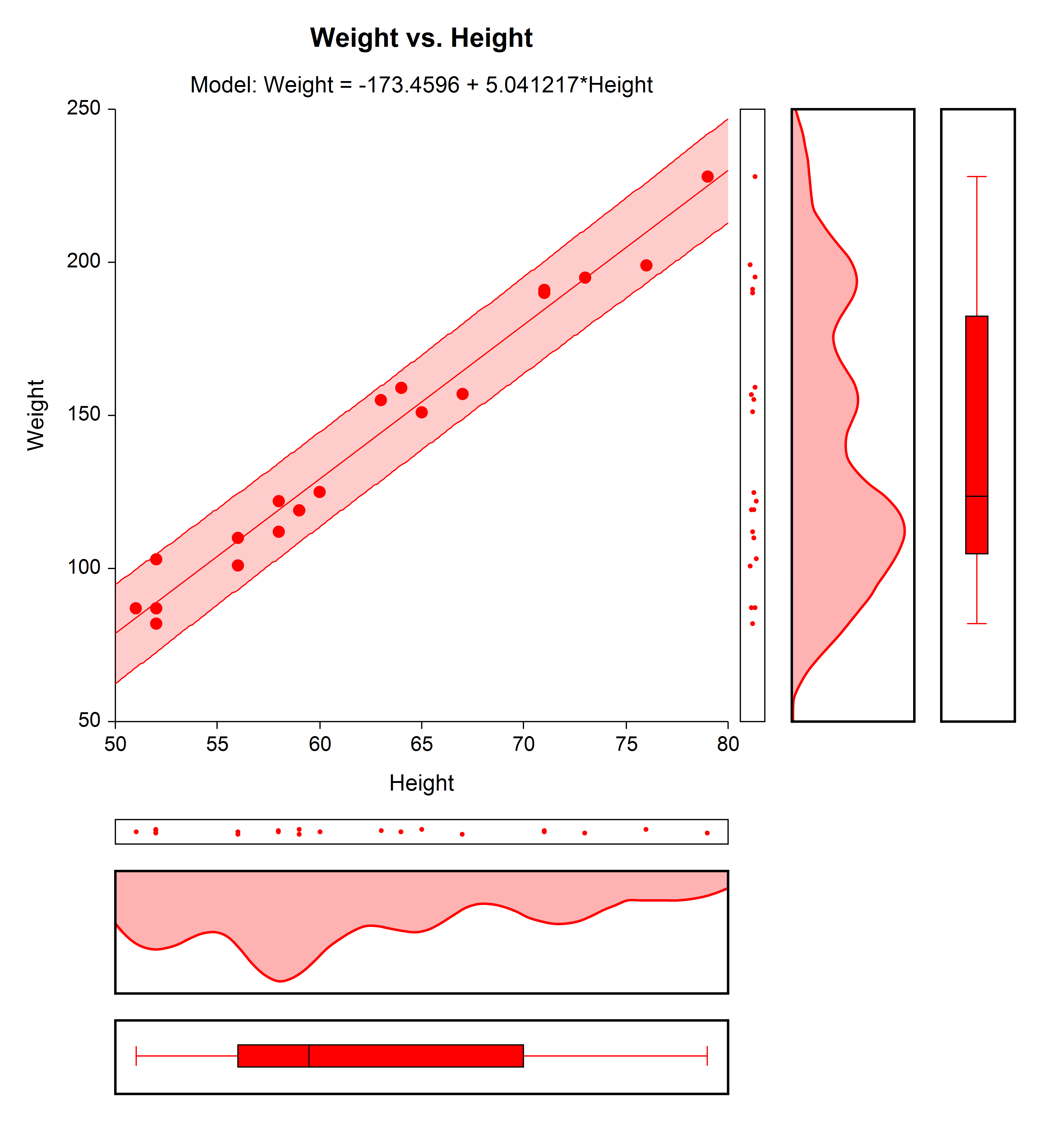A large number of specialized plots can also be produced in this procedure, such as Y vs. X plots, residual plots, RStudent vs. X plots, serial correlation plots, probability plots, and so forth.

Sample Data

Sample Output

Box-Cox Transformation for Simple Linear Regression

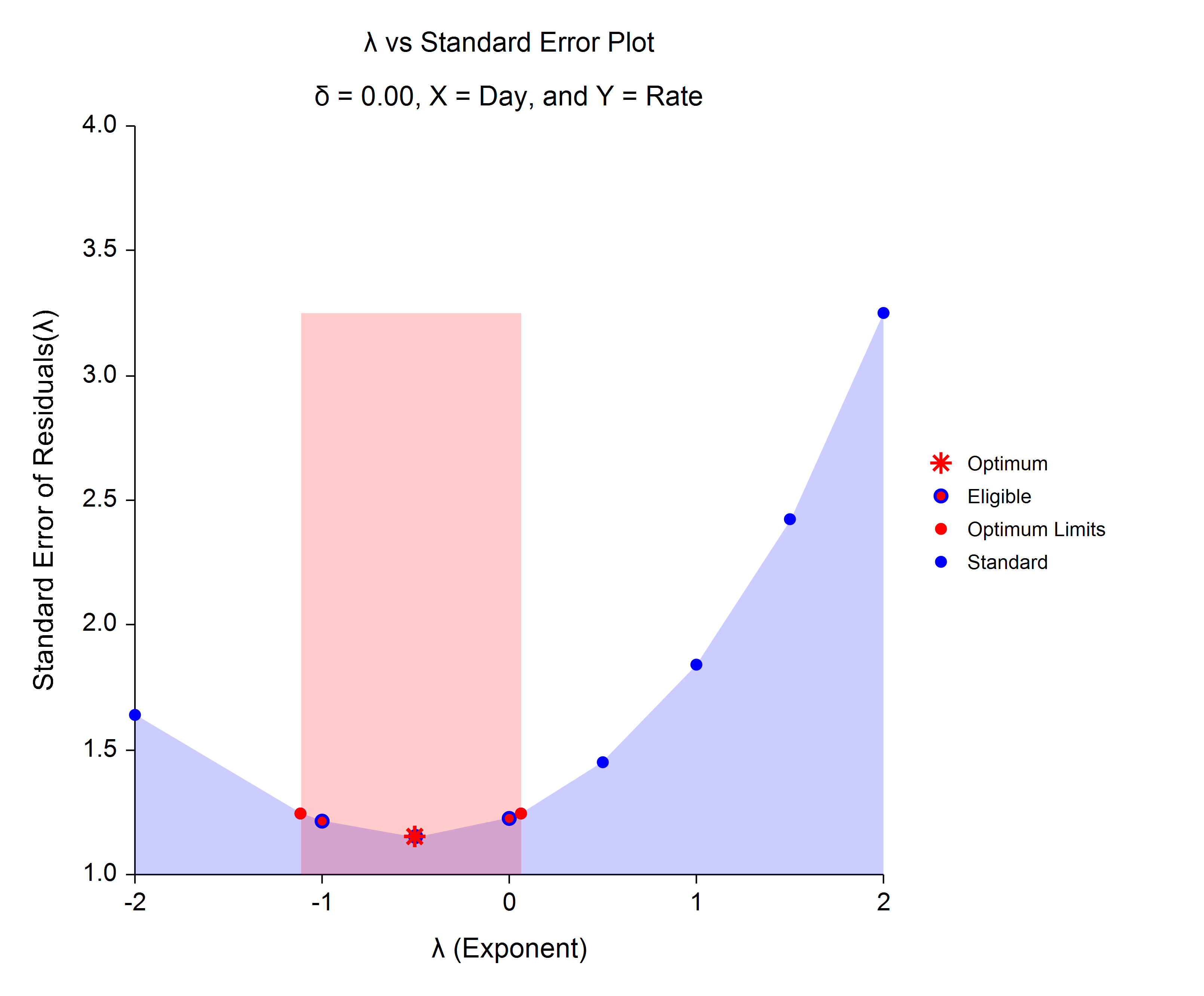
[Documentation PDF]

The Box-Cox Transformation refers to a method for finding an appropriate exponent to use to transform data to follow the normal distribution. The Box-Cox Transformation for Simple Linear Regression procedure in NCSS allows you to find an appropriate power-transformation exponent such that the residuals from simple linear regression are normally distributed, which is a key assumption in regression. The procedure finds the optimum maximum likelihood exponent and automatically calculates a confidence interval. The procedure also automatically tests the residuals for normality after fitting the linear regression model using the optimum exponent. The following is an example plot produced by this procedure demonstrating the properties of various possible transformation exponents. In the example, the optimum power transformation has an exponent of about -0.5 (i.e. 1/Square Root(X)).

Box-Cox Exponent (λ) Plot

Robust Linear Regression (Passing-Bablok Median-Slope)

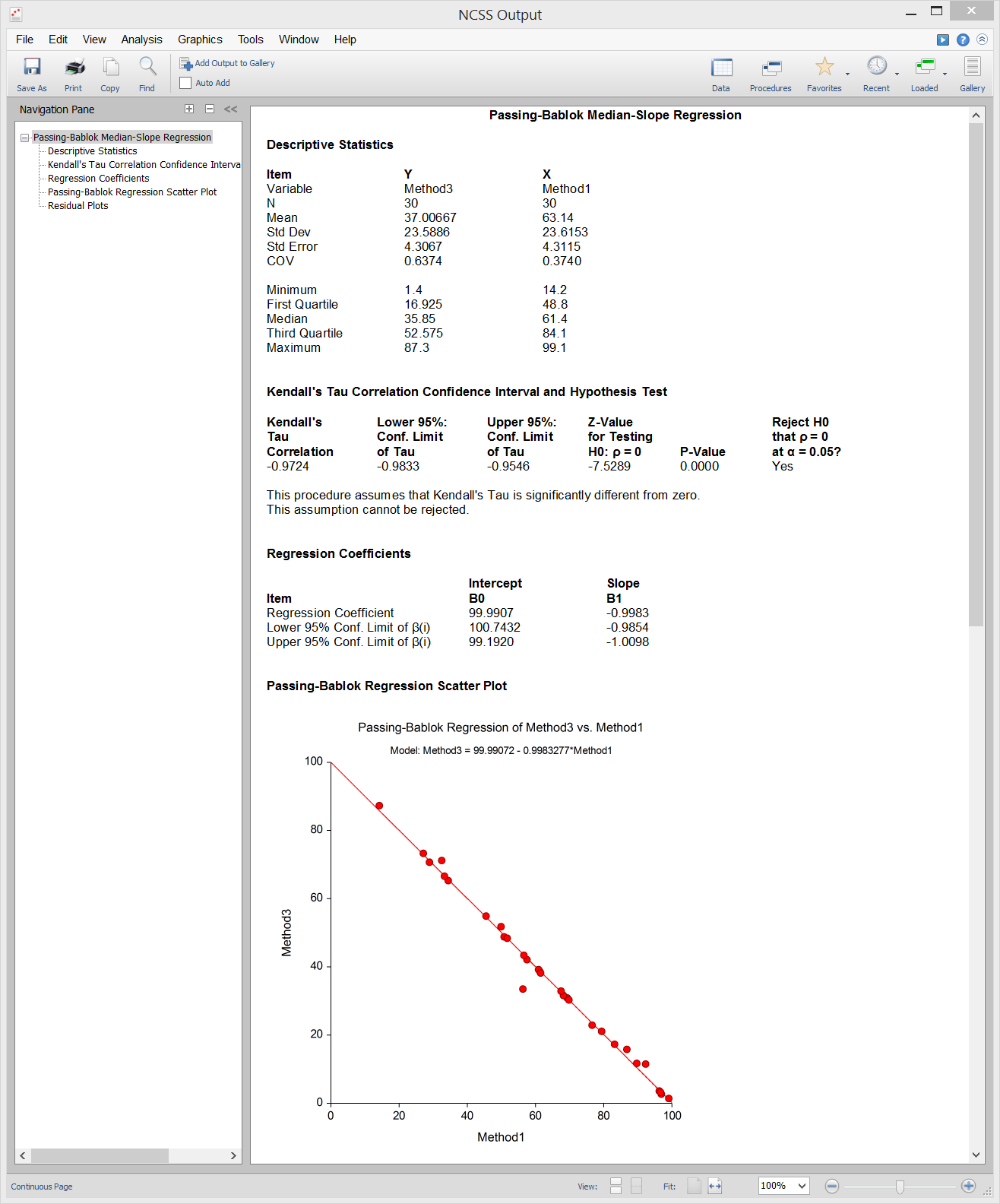
[Documentation PDF]

The Passing-Bablok Median-Slope algorithm can be applied in a simple linear regression setting to come up with a robust estimator of the intercept and slope in the regression equation. The regression slope (?₁) estimate is calculated as the median of all slopes that can be formed from all of the possible data point pairs, except those that result in an undefined slope of 0/0. The intercept (?₀) estimate is the median of all {Yi – ?₁ * Xi}. This method is often used for transference, where a reference interval is rescaled.

Sample Output

Multiple Regression

Multiple Linear Regression refers to the case where there are multiple explanatory X variables and one continuous dependent Y variable in the regression model. The multiple linear regression model equation for k variables is of the form

Y = ?₀ + ?₁* X₁ + ?₂* X₂ + … + ?_k* X_k.

NCSS includes several procedures involving various multiple linear regression methods:

• 1. Multiple Regression
• 2. Multiple Regression - Basic
• 3. Multiple Regression for Appraisal
• 4. Multiple Regression with Serial Correlation
• 5. Principal Components Regression
• 6. Response Surface Regression
• 7. Ridge Regression
• 8. Robust Regression

Multiple Regression

[Documentation PDF]

Multiple Regression refers to a set of techniques for studying the relationship between a numeric dependent variable and one or more independent variables based on a sample. The Multiple Regression analysis procedure in NCSS computes a complete set of statistical reports and graphs commonly used in multiple regression analysis. The Multiple Regression – Basic procedure eliminates many of the advanced multiple regression reports and inputs to focus on the most widely-used analysis reports and graphs. The Multiple Regression for Appraisal procedure presents the setup and reports in a manner that is relevant for appraisers. The Multiple Regression with Serial Correlation procedure contains methods (i.e. the Cochrane-Orcutt procedure) for adjusting for serial correlation among observations as described here.

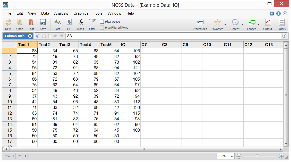
Data

NCSS is designed to work with both numeric and categorical independent variables. ‘Dummy’ variables for categorical independent variables are created internally based on any of a number of recoding schemes.

The Regression Model

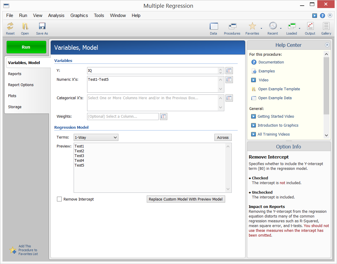
Regression models up to a certain order can be defined using a simple drop-down, or a flexible custom model may be entered. NCSS maintains groups of ‘dummy’ variables associated with a categorical independent variable together, to make analysis and interpretation of these variables much simpler.

Sample Data

Procedure Input

Sample Output

The output includes summary statistics, hypothesis tests and probability levels, confidence and prediction intervals, and goodness-of-fit information. Additional diagnostics include PRESS statistics, normality tests, the Durbin-Watson test, R-Squared, multicollinearity analysis, DFBETAS, eigenvalues, and eigenvectors. An extensive set of graphs for analysis of residuals are also available.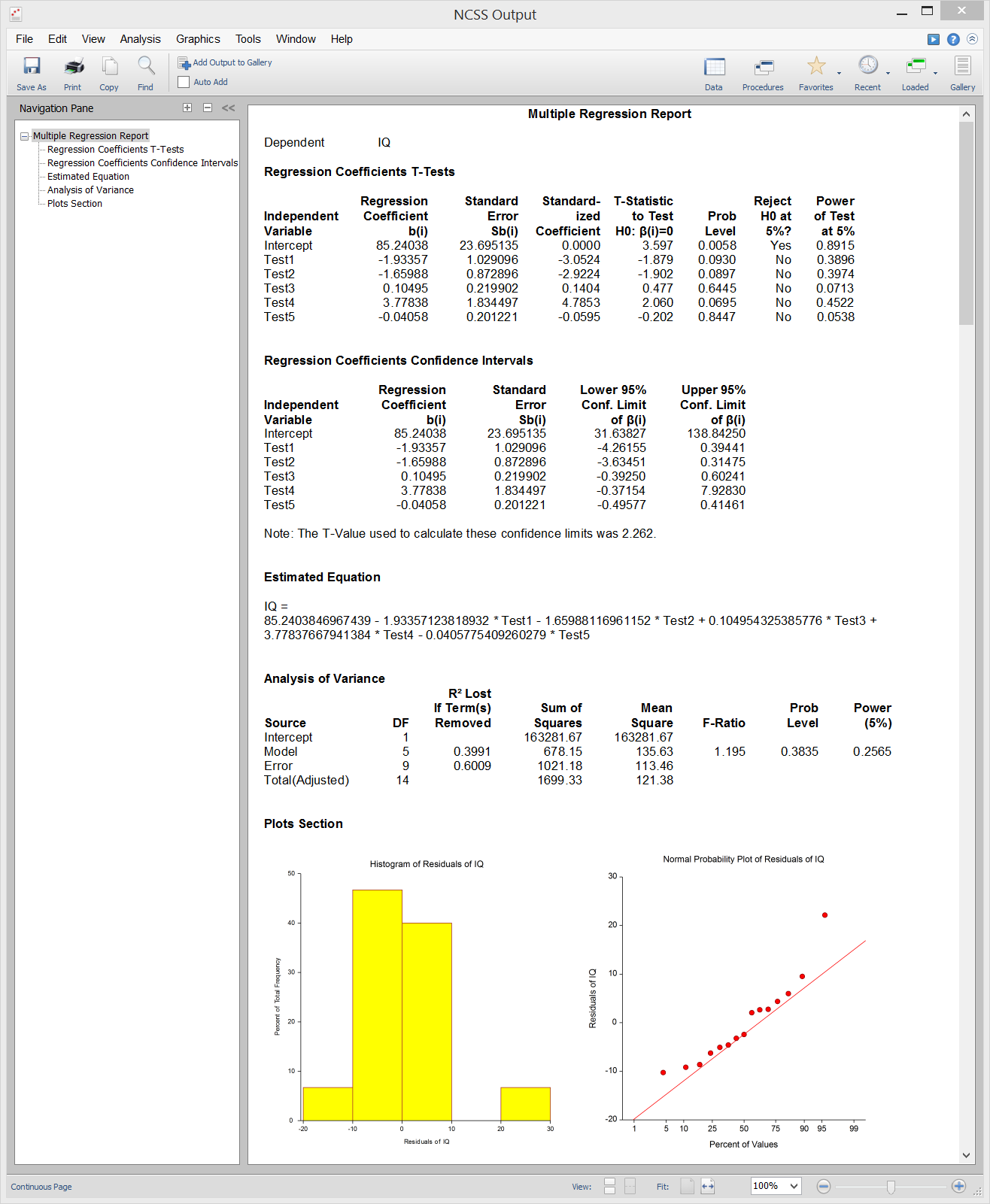

Some Plots from a Typical Multiple Regression Analysis in NCSS

Principal Components Regression

<a href="https://www.ncss.com/wp-content/themes/ncss/pdf/Procedures/NCSS/[Documentation PDF]

.pdf" target=_blank>[Documentation PDF]

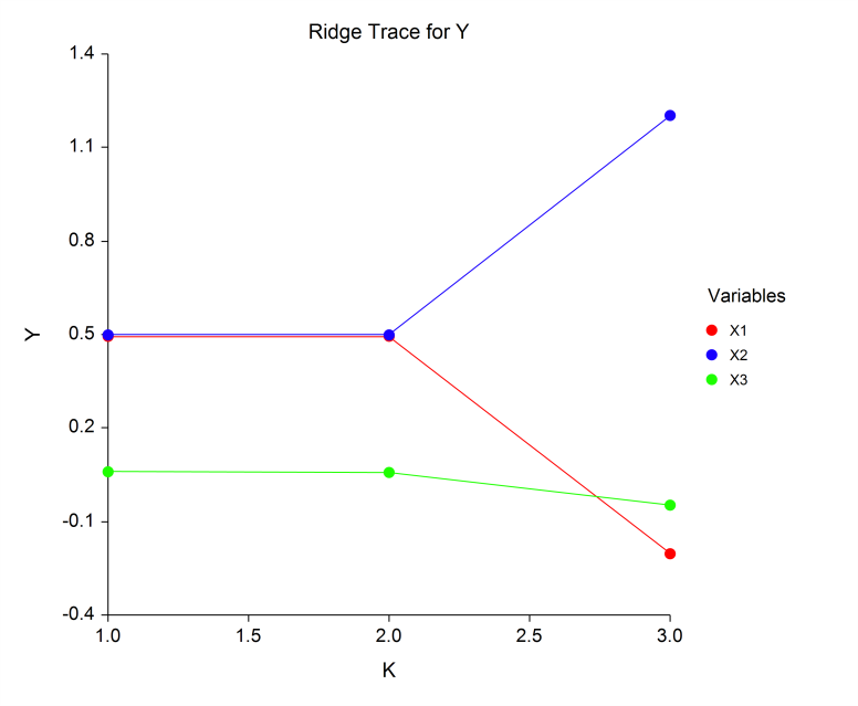
Principal components regression is a technique for analyzing multiple regression data that suffer from multicollinearity. When multicollinearity occurs, least squares estimates are unbiased, but their variances are large so they may be far from the true value. By adding a degree of bias to the regression estimates, principal components regression reduces the standard errors. It is hoped that the net effect will be to give more reliable estimates.

Some Plots from a Principal Components Regression Analysis in NCSS

Response Surface Regression

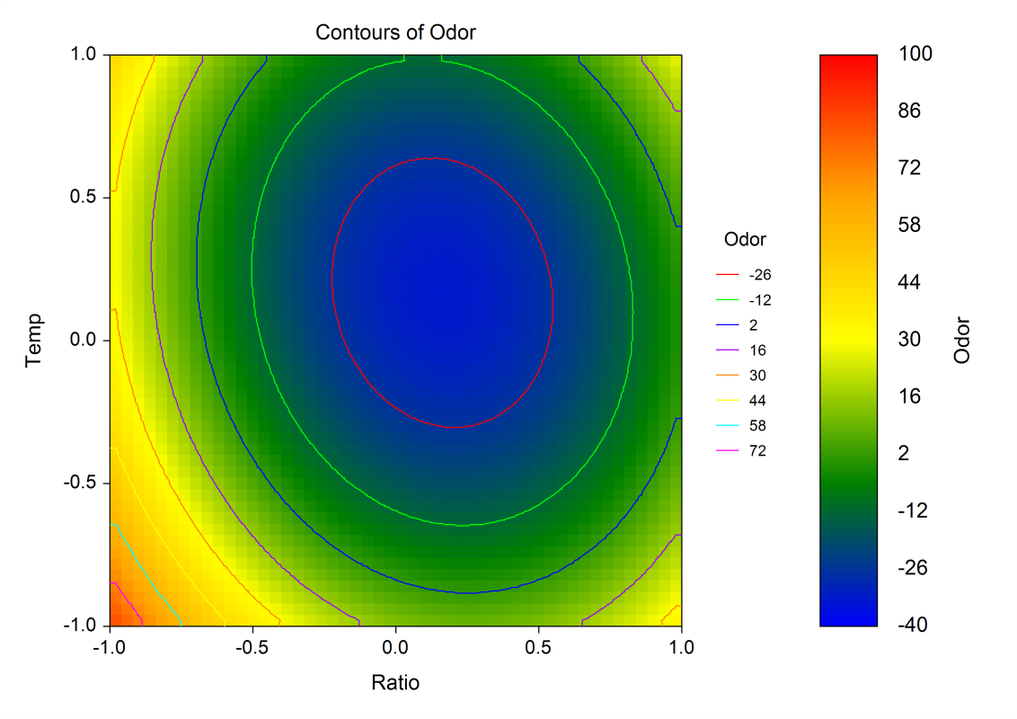
[Documentation PDF]

The Response Surface Regression procedure in NCSS uses response surface analysis to fit a polynomial regression model with cross-product terms of variables that may be raised up to the third power. It calculates the minimum or maximum of the surface. The program also has a variable selection feature that helps you find the most parsimonious hierarchical model. NCSS automatically scans the data for duplicates so that a lack-of-fit test may be calculated using pure error. One of the main goals of response surface analysis is to find a polynomial approximation of the true nonlinear model, similar to the Taylor’s series expansion used in calculus. Hence, you are searching for an approximation that works well in a specified region. As the region is reduced, the number of terms may also be reduced. In a very small region, a linear (first-order) approximation may be adequate. A larger region may require a quadratic (second-order) approximation.

A Contour Plot from a Response Surface Regression Analysis in NCSS

Ridge Regression

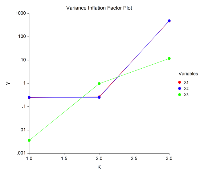
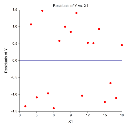
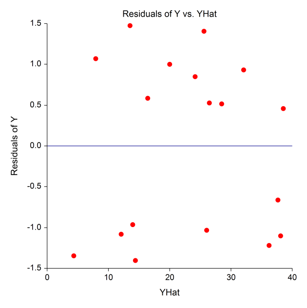
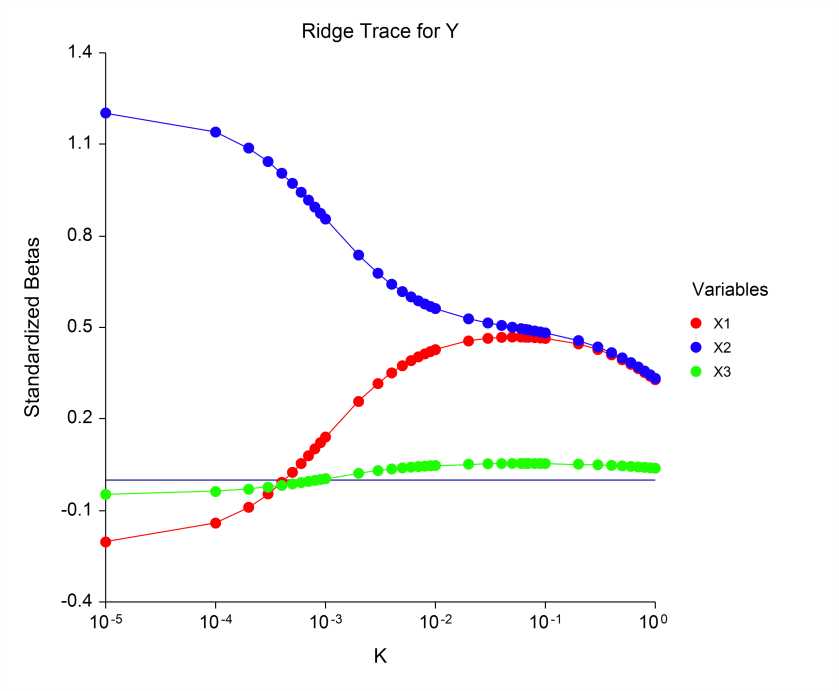
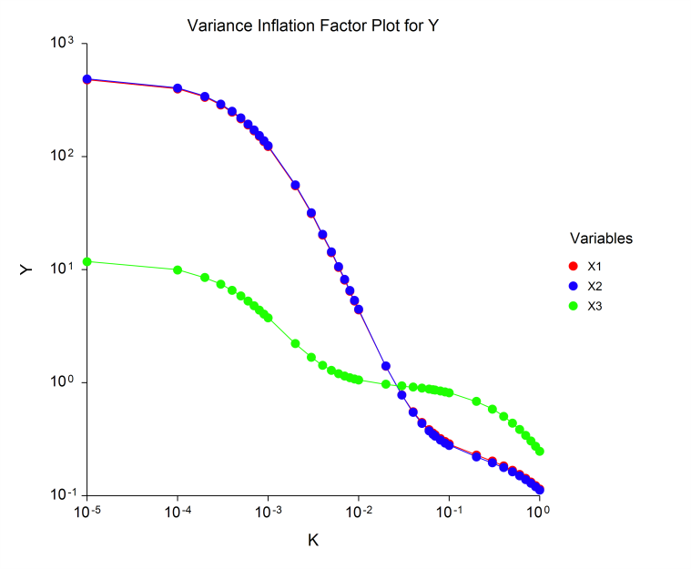
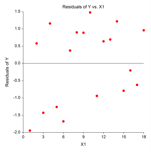
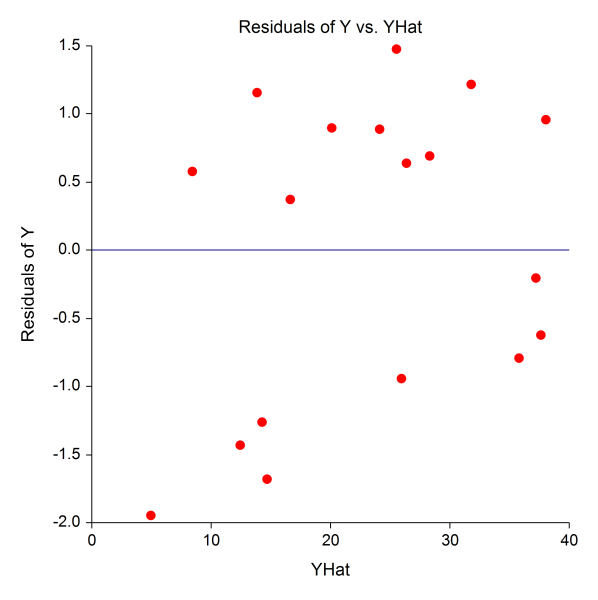
[Documentation PDF]

Ridge regression is a technique for analyzing multiple regression data that suffer from multicollinearity. When multicollinearity occurs, least squares estimates are unbiased, but their variances are large so they may be far from the true value. By adding a degree of bias to the regression estimates, it is anticipated that the net effect will be to give more reliable estimates. The Ridge Regression procedure in NCSS provides results on the least squares multicollinearity, the eigenvalues and eigenvectors of the correlations, ridge trace and variance inflation factor plots, standardized ridge regression coefficients, K analysis, ridge versus least squares comparisons, analysis of variance, predicted values, and residual plots.

Some Plots from a Ridge Regression Analysis in NCSS

Robust Regression

[Documentation PDF]

Robust regression provides an alternative to least squares regression that works with less restrictive assumptions. Specifically, it provides much better regression coefficient estimates when outliers are present in the data. Outliers violate the assumption of normally distributed residuals in least squares regression. They tend to distort the least squares coefficients by having more influence than they deserve. Typically, you would expect that the weight attached to each observation would be about 1/N in a dataset with N observations. However, outlying observations may receive a weight of 10, 20, or even 50%. This leads to serious distortions in the estimated coefficients. Because of this distortion, these outliers are difficult to identify since their residuals are much smaller than they should be. When only one or two independent variables are used, these outlying points may be visually detected in various scatter plots. However, the complexity added by additional independent variables often hides the outliers from view in scatter plots. Robust regression down-weights the influence of outliers. This makes residuals of outlying observations larger and easier to spot. Robust regression is an iterative procedure that seeks to identify outliers and minimize their impact on the coefficient estimates. The amount of weighting assigned to each observation in robust regression is controlled by a special curve called an influence function. There are two influence functions available in NCSS. Although robust regression can be very beneficial when used properly, careful consideration should be given to the results. Essentially, robust regression conducts its own residual analysis and down-weights or completely removes various observations. You should study the weights it assigns to each observation, determine which observations have been largely eliminated, and decide if these observations should be included in the analysis. The Robust Regression procedure in NCSS provides all the necessary output for a standard robust regression analysis.

Logistic Regression

Logistic Regression is used to study the association between multiple explanatory X variables and one categorical dependent Y variable. NCSS includes two logistic regression procedures:

• 1. Logistic Regression
• 2. Conditional Logistic Regression

Logistic Regression

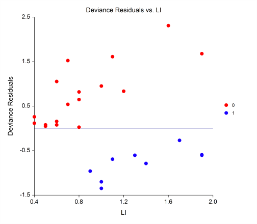
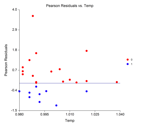
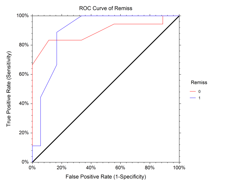
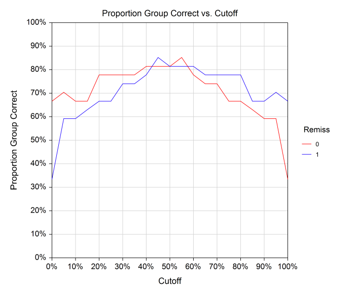
[Documentation PDF]

Logistic regression is used when the dependent variable is categorical rather than continuous. In most cases where logistic regression is used, the dependent variable is binary (yes/no, present/absent, positive/negative, etc.), but if the response has more than two categories, the Logistic Regression procedure in NCSS can still be used. This special case is sometimes called multinomial logistic regression or multiple group logistic regression. The Logistic Regression procedure in NCSS provides a full set of analysis reports, including response analysis, coefficient tests and confidence intervals, analysis of deviance, log-likelihood and R-Squared values, classification and validation matrices, residual diagnostics, influence diagnostics, and more. This procedure also gives Y vs. X plots, deviance and Pearson residual plots, ROC curves. It can conduct an independent variable subset selection using the latest stepwise search algorithms.

Sample Output

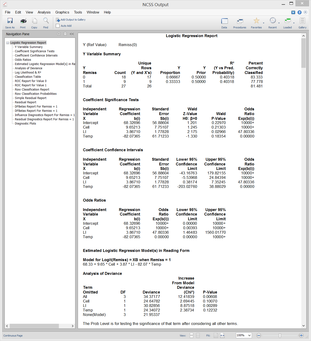
Some Residual and ROC Plots from a Logistic Regression Analysis in NCSS

 

Conditional Logistic Regression

[Documentation PDF]

Conditional logistic regression (CLR) is a specialized type of logistic regression that is usually employed when case subjects with a particular condition or attribute are each matched with n control subjects without the condition. In general, there may be 1 to m cases matched with 1 to n controls, however, the most common design utilizes 1:1 matching.

Nonlinear Regression

NCSS includes several procedures for nonlinear regression and curve fitting:

• 1. Nonlinear Regression
• 2. Curve Fitting - General
• 3. Michaelis-Menten Equation
• 4. Sum of Functions Models
• 5. Fractional Polynomial Regression
• 6. Ratio of Polynomials Fit - One Variable
• 7. Ratio of Polynomials Search - One Variable
• 8. Harmonic Regression
• 9. Ratio of Polynomials Fit - Many Variables
• 10. Ratio of Polynomials Search - Many Variables

Nonlinear Regression

[Documentation PDF]

Multiple regression deals with models that are linear in the parameters. That is, the multiple regression model may be thought of as a weighted average of the independent variables. A linear model is usually a good first approximation, but occasionally, you will require the ability to use more complex, nonlinear, models. Nonlinear regression models are those that are not linear in the parameters. Examples of nonlinear equations are:

Y = A + B EXP(‑CX)

Y = (A + BX)/(1 + CX)

Y = A + B/(C + X)

The Nonlinear Regression procedure in NCSS estimates the parameters in nonlinear models using the Levenberg-Marquardt nonlinear least-squares algorithm as presented in Nash (1987). We have implemented Nash’s MRT algorithm with numerical derivatives. This has been a popular algorithm for solving nonlinear least squares problems, since the use of numerical derivatives means you do not have to supply program code for the derivatives.

Starting Values

Many people become frustrated with the complexity of nonlinear regression after dealing with the simplicity of multiple linear regression analysis. Perhaps the biggest nuisance with the algorithm used in this program is the need to supply bounds and starting values. The convergence of the algorithm depends heavily upon supplying appropriate starting values. Sometimes you will be able to use zeros or ones as starting values, but often you will have to come up with better values. One accepted method for obtaining a good set of starting values is to estimate them from the data.

Assumptions and Limitations

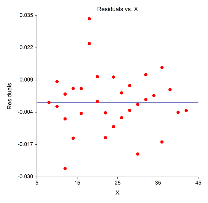
Usually, nonlinear regression is used to estimate the parameters in a nonlinear model without performing hypothesis tests. In this case, the usual assumption about the normality of the residuals is not needed. Instead, the main assumption needed is that the data may be well represented by the model.

A Residual Plot from a Nonlinear Regression Analysis in NCSS

Curve Fitting

[Documentation PDF]

Curve fitting refers to finding an appropriate mathematical model that expresses the relationship between a dependent variable Y and a single independent variable X (or group of X’s) and estimating the values of its parameters using nonlinear regression. Click here for more information about the curve fitting procedures in NCSS.

Regression for Method Comparison

Method comparison is used to determine if a new method of measurement is equivalent to a standard method currently in use. NCSS includes two regression procedures with application to method comparison:

• 1. Deming Regression
• 2. Passing-Bablok Regression

Deming Regression

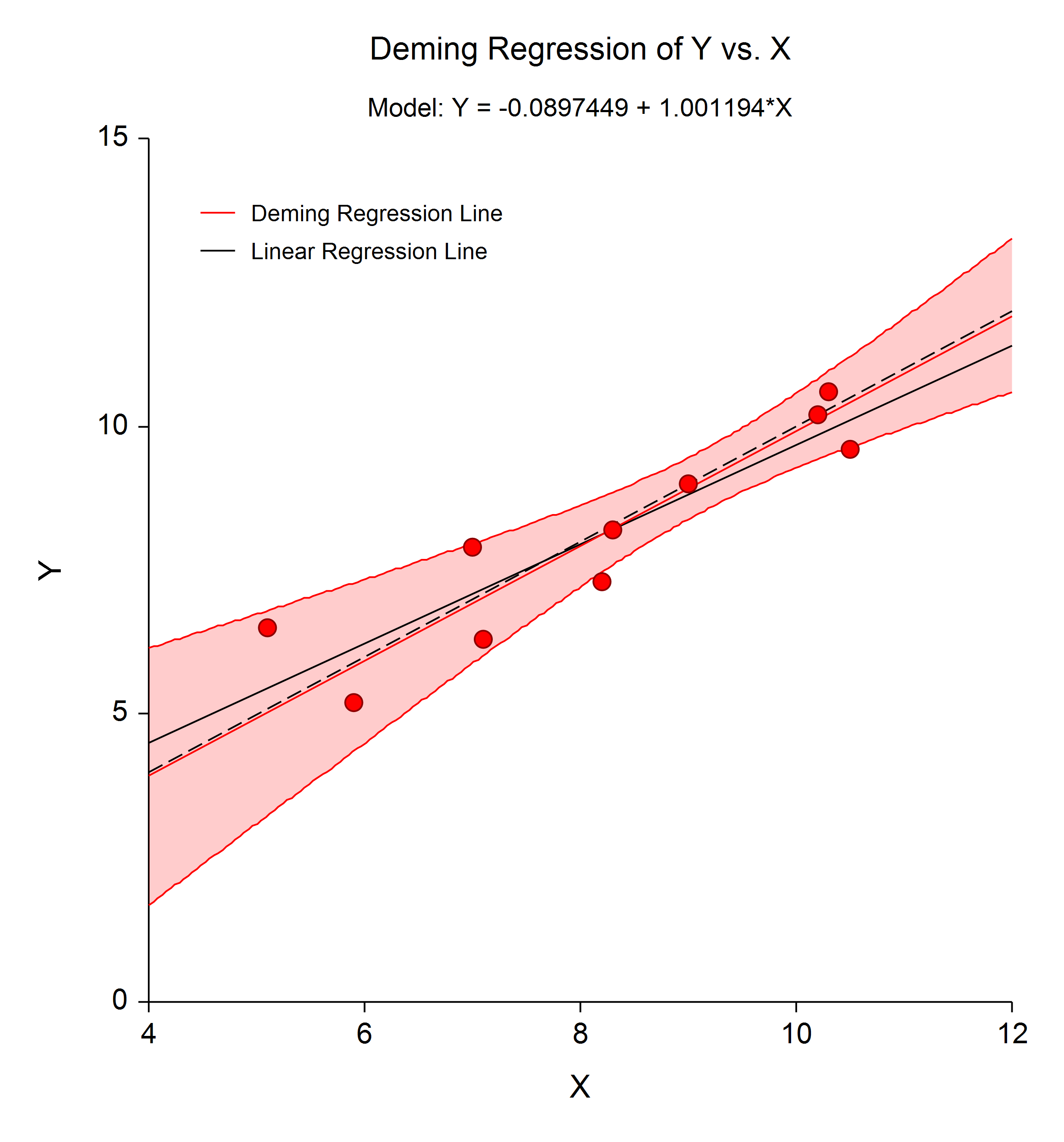
[Documentation PDF]

Deming regression is a technique for fitting a straight line to two-dimensional data where both variables, X and Y, are measured with error. Click here for more information about the Deming Regression procedure in NCSS.

Deming Regression Plot

Passing-Bablok Regression

[Documentation PDF]

Passing-Bablok Regression for method comparison is a robust, nonparametric method for fitting a straight line to two-dimensional data where both variables, X and Y, are measured with error. Click here for more information about the Passing-Bablok Regression procedure in NCSS.

Regression with Survival or Reliability Data

Survival and reliability data present a particular challenge for regression because it involves often-censored lifetime or survival data which is not normally distributed. NCSS includes two procedures that perform regression with survival data:

• 1. Cox (Proportional Hazards) Regression
• 2. Parametric Survival (Weibull) Regression

Cox (Proportional Hazards) Regression

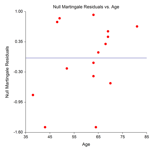
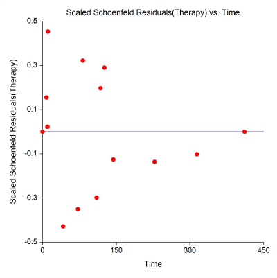
[Documentation PDF]

Cox regression is similar to regular multiple regression except that the dependent (Y) variable is the hazard rate. Cox regression is commonly used in determining factors relating to or influencing survival. As in the Multiple, Logistic, Poisson, and Serial Correlation Regression procedures, specification of both numeric and categorical independent variables is permitted. In addition to model estimation, Wald tests and confidence intervals of the regression coefficients, NCSS provides an analysis of deviance table, log likelihood analysis, and extensive residual analysis including Pearson and Deviance residuals. The Cox Regression procedure in NCSS can also be used conduct a subset selection of the independent variables using a stepwise-type search algorithm.

Residual Plots from a Cox Regression Analysis in NCSS

 

Parametric Survival (Weibull) Regression

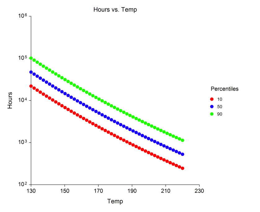
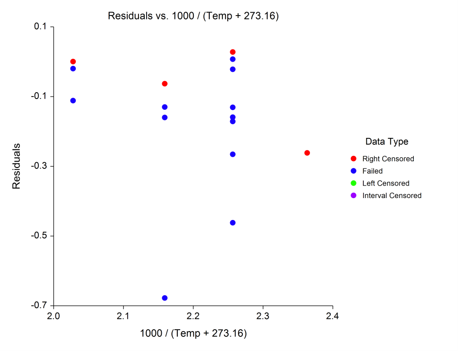
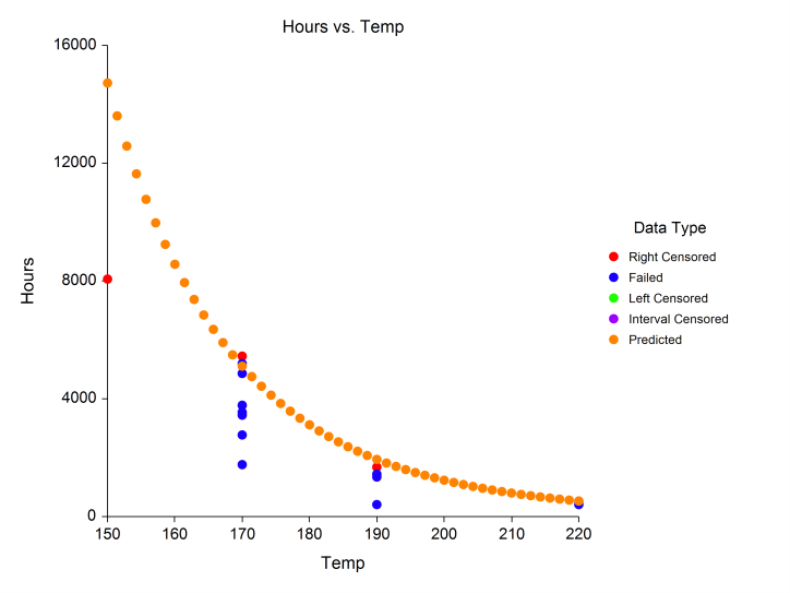
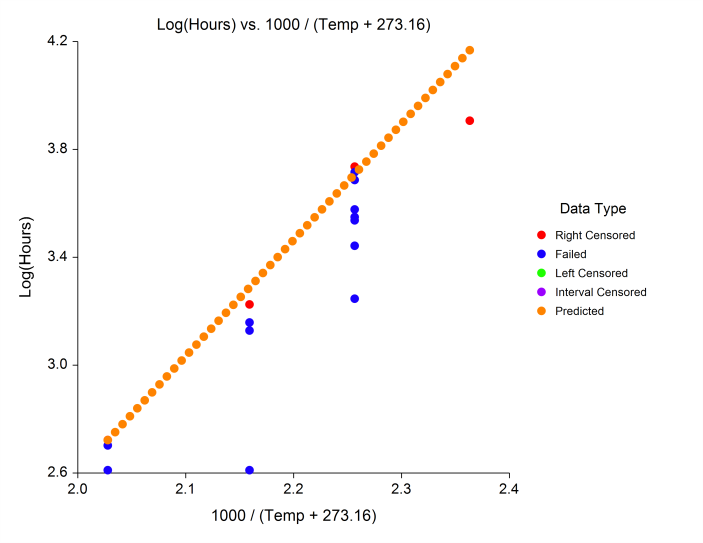
[Documentation PDF]

This procedure in NCSS fits the regression relationship between a positive-valued dependent variable (often time to failure) and one or more independent variables. The distribution of the residuals (errors) is assumed to follow the exponential, extreme value, logistic, log-logistic, lognormal, lognormal10, normal, or Weibull distribution. The data may include failed, left censored, right censored, and interval observations. This type of data often arises in the area of accelerated life testing. When testing highly reliable components at normal stress levels, it may be difficult to obtain a reasonable amount of failure data in a short period of time. For this reason, tests are conducted at higher than expected stress levels. The models that predict failure rates at normal stress levels from test data on items that fail at high stress levels are called acceleration models. The basic assumption of acceleration models is that failures happen faster at higher stress levels. That is, the failure mechanism is the same, but the time scale has been shortened.

Plots from a Parametric Survival (Weibull) Regression Analysis in NCSS

Regression with Count Data

When the regression data involves counts, the data often follows a Poisson or Negative Binomial distribution (or variant of the two) and must be modeled appropriately for accurate results. The possible values of Y are the nonnegative integers: 0, 1, 2, 3, and so on. NCSS includes five procedures that can be used to model count data:

• 1. Poisson Regression
• 2. Zero-Inflated Poisson Regression
• 3. Negative Binomial Regression
• 4. Zero-Inflated Negative Binomial Regression
• 5. Geometric Regression

Poisson Regression

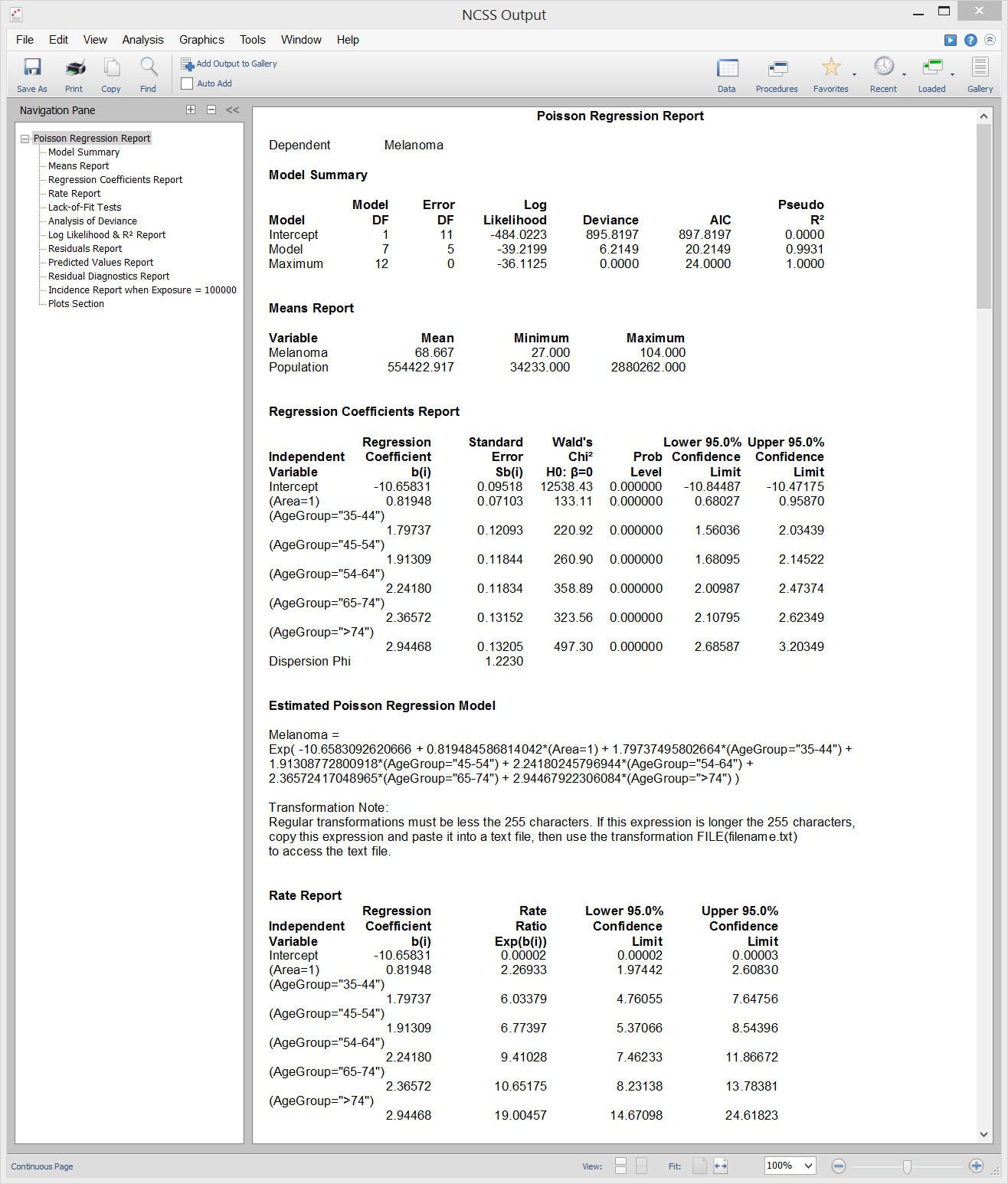
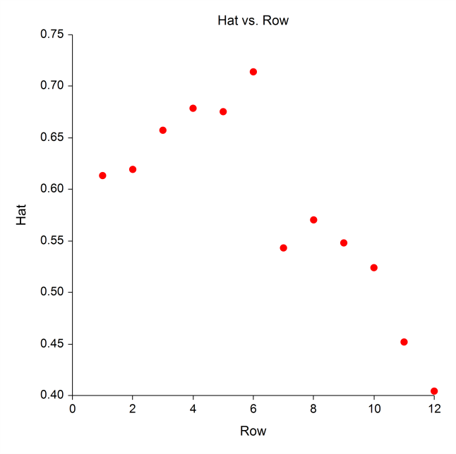
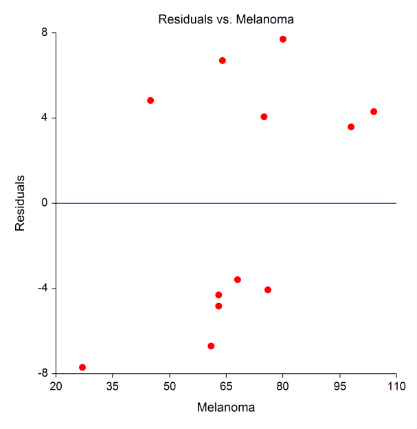
[Documentation PDF]

Poisson regression is similar to regular multiple regression analysis except that the dependent (Y) variable is a count that is assumed to follow the Poisson distribution. Both numeric and categorical independent variables may specified, in a similar manner to that of the Multiple Regression procedure. The Poisson Regression procedure in NCSS provides an analysis of deviance table, log likelihood analysis, and as well as the necessary coefficient estimates and Wald tests. It also provides extensive residual analysis including Pearson and Deviance residuals. Subset selection of the independent variables using a stepwise-type searching algorithm can also be performed in this procedure.

Sample Output

Residual Plots from a Poisson Regression Analysis in NCSS

  

Zero-Inflated Poisson Regression

[Documentation PDF]

The Zero-Inflated Poisson Regression procedure is used for count data that exhibit excess zeros and overdispersion. The distribution of the data combines the Poisson distribution and the logit distribution. The procedure computes zero-inflated Poisson regression for both continuous and categorical variables. It reports on the regression equation, confidence limits, and the likelihood. It also performs comprehensive residual analysis, including diagnostic residual reports and plots.

Negative Binomial Regression

[Documentation PDF]

Negative Binomial Regression is similar to regular multiple regression except that the dependent variable (Y) is an observed count that follows the negative binomial distribution. Negative binomial regression is a generalization of Poisson regression which loosens the restrictive assumption that the variance is equal to the mean, as is required by the Poisson model. The traditional negative binomial regression model, commonly known as NB2, is based on the Poisson-gamma mixture distribution. This formulation is popular because it allows the modelling of Poisson heterogeneity using a gamma distribution. This procedure computes negative binomial regression for both continuous and categorical variables. It reports on the regression equation, goodness of fit, confidence limits, likelihood, and the model deviance. It performs a comprehensive residual analysis including diagnostic residual reports and plots. It can perform a subset selection search, looking for the best regression model with the fewest independent variables. It also provides confidence intervals for predicted values.

Zero-Inflated Negative Binomial Regression

[Documentation PDF]

The Zero-Inflated Negative Binomial Regression procedure is used for count data that exhibit excess zeros and overdispersion. The distribution of the data combines the negative binomial distribution and the logit distribution. The procedure computes zero-inflated negative binomial regression for both continuous and categorical variables. It reports on the regression equation, confidence limits, and the likelihood. It also performs comprehensive residual analysis, including diagnostic residual reports and plots.

Geometric Regression

[Documentation PDF]

Geometric Regression is a special case of negative binomial regression in which the dispersion parameter is set to one. It is similar to regular multiple regression except that the dependent variable (Y) is an observed count that follows the geometric distribution. Geometric regression is a generalization of Poisson regression which loosens the restrictive assumption that the variance is equal to the mean as is made by the Poisson model. This procedure computes geometric regression for both continuous and categorical variables. It reports on the regression equation, goodness of fit, confidence limits, likelihood, and deviance. It performs a comprehensive residual analysis including diagnostic residual reports and plots. It can perform a subset selection search, looking for the best regression model with the fewest independent variables. It also provides confidence intervals for predicted values.

Regression with Time Series Data

One of the basic requirements of regular multiple regression is that the observations are independent of one another. For time series data, this is not the case. NCSS includes two procedures for regression with serially correlated time series data:

• 1. Multiple Regression with Serial Correlation
• 2. Harmonic Regression

Multiple Regression with Serial Correlation

[Documentation PDF]

This procedure uses the Cochrane-Orcutt method to adjust for serial correlation when performing multiple regression. The regular Multiple Regression routine assumes that the random-error components are independent from one observation to the next. However, this assumption is often not appropriate for business and economic data. Instead, it may be more appropriate to assume that the error terms are positively correlated over time. Consequences of the error terms being serially correlated include inefficient estimation of the regression coefficients, under estimation of the error variance (MSE), under estimation of the variance of the regression coefficients, and inaccurate confidence intervals. The presence of serial correlation can be detected by the Durbin-Watson test and by plotting the residuals against their lags.

Sample Output

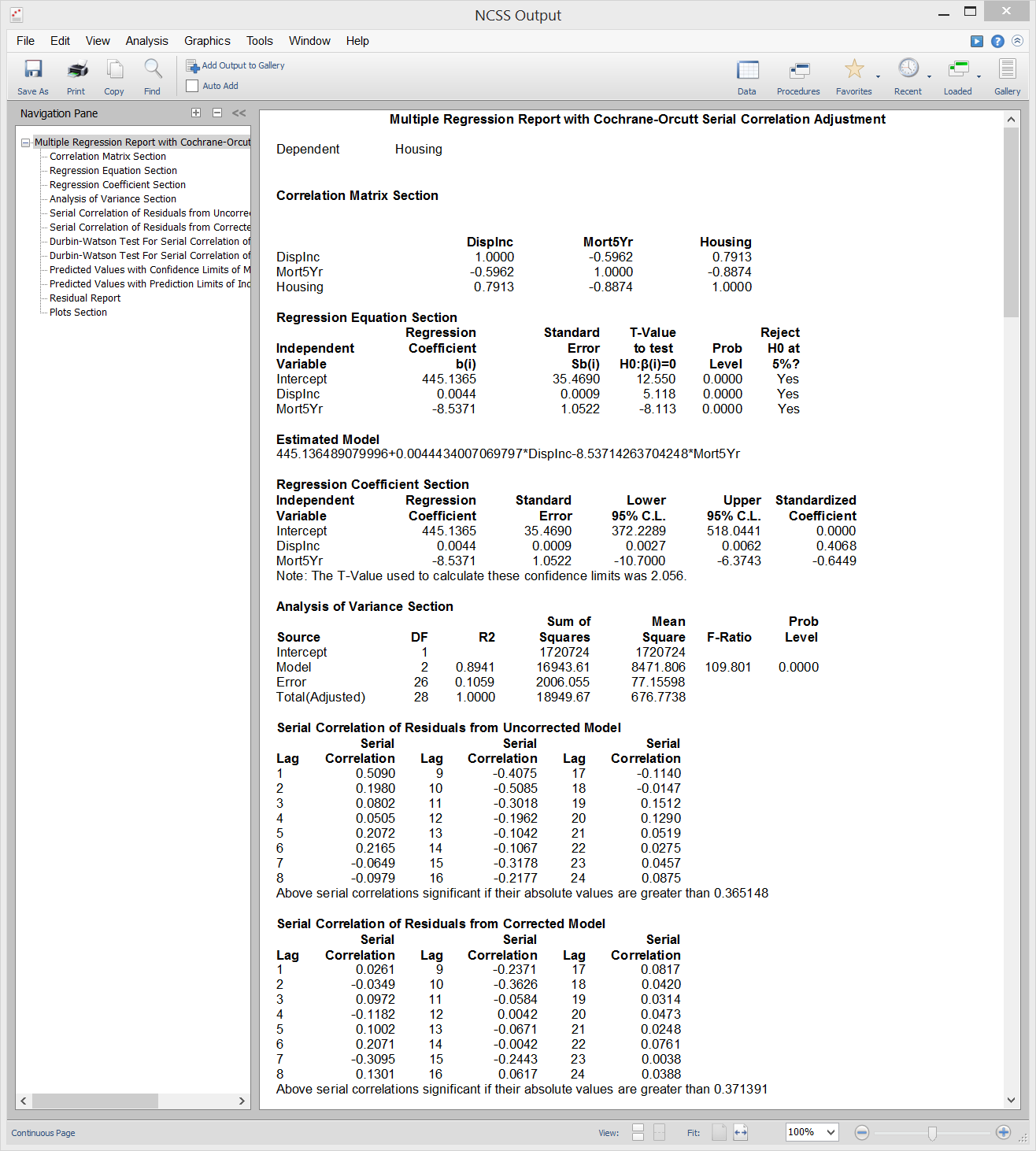
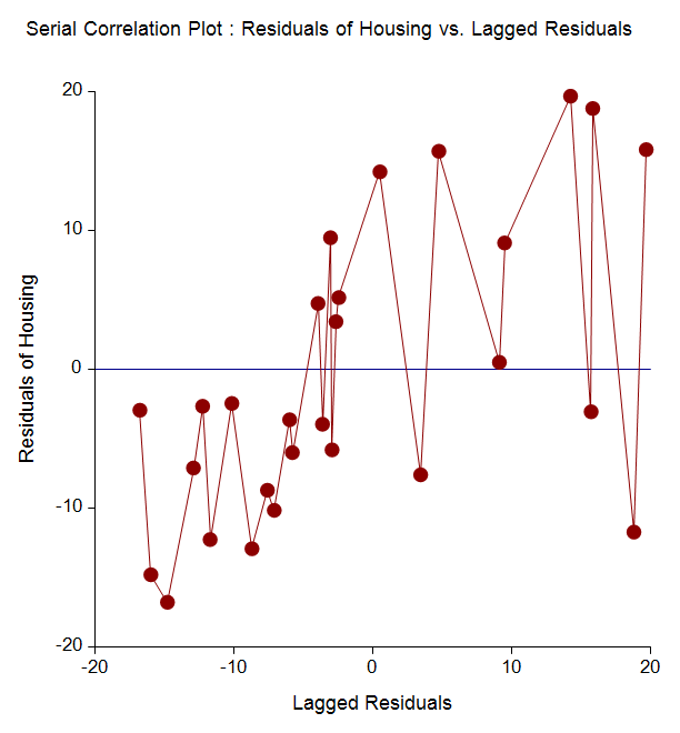
Serial Correlation Plot from a Multiple Regression with Serial Correlation Analysis in NCSS

Harmonic Regression

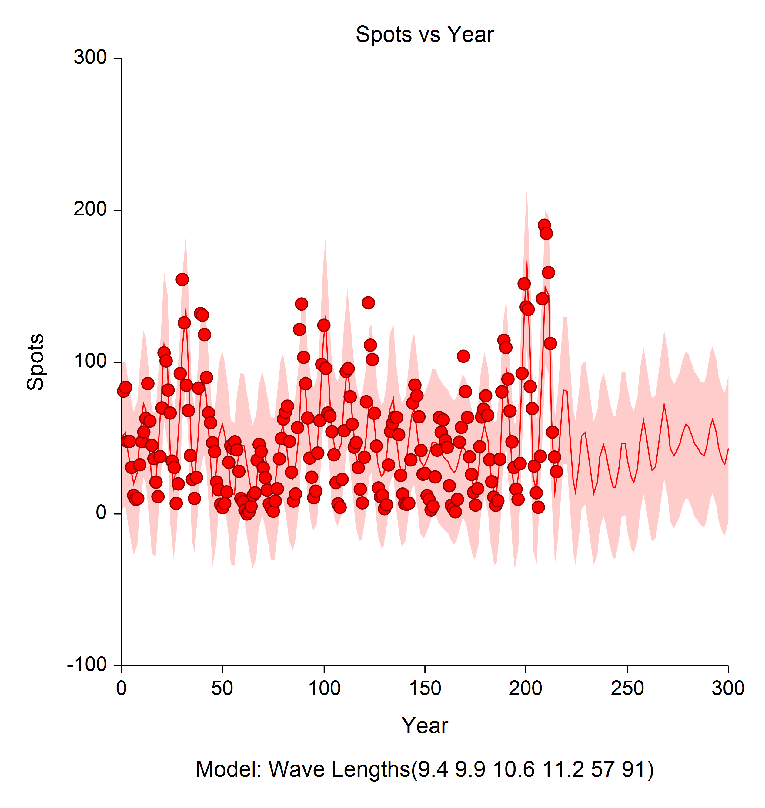
[Documentation PDF]

The Harmonic Regression procedure calculates the harmonic regression for time series data. To accomplish this, it fits designated harmonics (i.e. sinusoidal terms of different wavelengths) using nonlinear regression algorithms and automatically generates useful reports and plots specific to time series data.

Plot from Harmonic Regression Analysis in NCSS

Regression with Nondetects Data

The Nondetects-Data Regression procedure fits the regression relationship between a positive-valued dependent variable (with, possibly, some nondetected responses) and one or more independent variables. Click here for more information about the Nondetects-Data Regression procedure in NCSS.

Two-Stage Least Squares

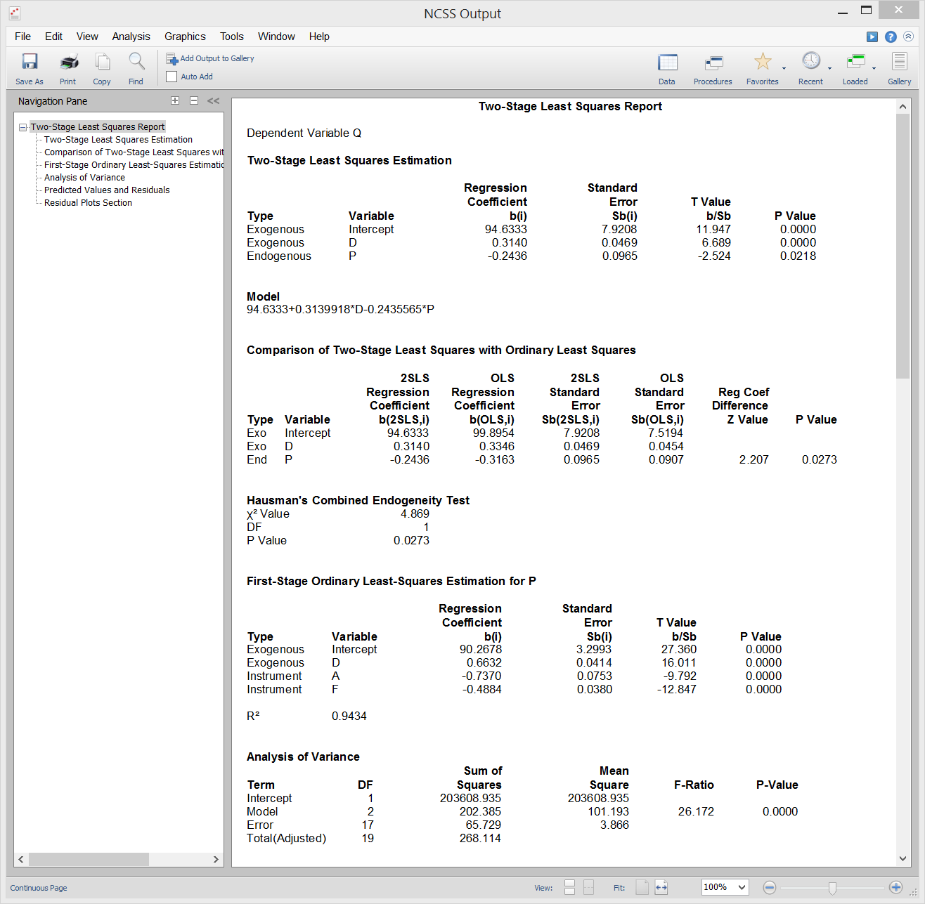
[Documentation PDF]

The Two-Stage Least Squares (2SLS) method available in NCSS is used fit models that include four types of variable(s): dependent, exogenous, endogenous, and instrument. These variables are defined and used as follows: A Dependent Variable is the response variable (Y) that is to be regressed on the exogenous and endogenous (but not the instrument) variables. The Exogenous Variables are independent variables that are included in both the first and second stage regression models. They are not correlated with the random error values in the second stage regression. The Endogenous Variables become the dependent variable in the first stage regression equation. Each is regressed on all exogenous and instrument variables. The predicted values from these regressions replace the original values of the endogenous variables in the second stage regression model. Two-Stage Least Squares is used in econometrics, statistics, and epidemiology to provide consistent estimates of a regression equation when controlled experiments are not possible.

Sample Output

Subset Selection

Often theory and experience give only general direction as to which of a pool of candidate variables should be included in the regression model. The actual set of predictor variables used in the final regression model must be determined by analysis of the data. Determining this subset is called the variable selection problem. Finding this subset of regressor (independent) variables involves two opposing objectives. First, we want the regression model to be as complete and realistic as possible. We likely want every regressor that is even remotely related to the dependent variable to be included. Second, we want to include as few variables as possible because each irrelevant regressor decreases the precision of the estimated coefficients and predicted values. Also, the presence of extra variables increases the complexity of data collection and model maintenance. The goal of variable selection becomes one of parsimony: achieve a balance between simplicity (as few regressors as possible) and fit (as many regressors as needed). A number of procedures are available in NCSS for determining the appropriate set of terms that should be included in your regression model.

Subset Selection in Multiple Regression

In NCSS, there are three procedures for subset selection in multiple regression.

• Subset Selection in Multiple Regression
• All Possible Regressions
• Stepwise Regression

The Subset Selection in Multiple Regression procedure has various forward selection methods including hierarchical forward selection, where interaction terms are included only if all terms of a lesser degree are included. This procedure is also especially useful when categorical variables are in the model, as it keeps the dummy variables associated with the categorical variables together. This procedure also provides a regression analysis for the final model of the search. [Documentation PDF]

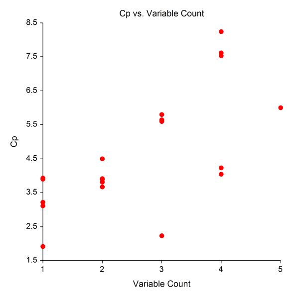
The All Possible Regressions procedure provides an exhaustive search of all possible combinations of up to 15 independent variables. The top models for each number of independent variables are displayed in order according to the criterion of interest (R-Squared or Root MSE). R-Squared, Root MSE, and Cp Plots can also be generated. [Documentation PDF]

When selecting among a large number of candidate independent variables, the Stepwise Regression procedure may be used to determine a reasonable subset. Three selection methods are available in this procedure. [Documentation PDF]

Forward (Step-Up) Selection

The forward selection method begins with no candidate variables in the model. The variable that has the highest R-Squared is chosen first. At each step, the candidate variable that increases R-Squared the most is selected. Variable addition stops when none of the remaining variables meet the specified significance criterion. In this method, once a variable enters the model, it cannot be deleted.

Backward (Step-Down) Selection

The backward selection model starts with all candidate variables in the model. At each step, the variable that is the least significant is removed. This process continues until only variables with the user-specified significance remain in the model.

Stepwise Selection

Stepwise regression is a combination of the forward and backward selection techniques. In this method, after each step in which a variable was added, all candidate variables in the model are checked to determine if their significance has been reduced below the specified level. If a nonsignificant variable is found, it is removed from the model. Stepwise regression requires two significance levels: one for adding variables and one for removing variables.

Subset Selection in Logistic, Conditional Logistic, Cox, Poisson, Negative Binomial, and Geometric Regression

Built into the Logistic, Conditional Logistic, Cox, Poisson, Negative Binomial, and Geometric Regression analysis procedures is the ability to also perform subset selection. In each of these procedures, subset selection can be performed with both numeric and categorical variables, where the dummy variables associated with each categorical variable are maintained as a group. Search methods include Forward, Forward with Switching, Hierarchical Forward, and Hierarchical Forward with Switching.

Subset Selection in Multivariate Y Multiple Regression

[Documentation PDF]

For the case where multiple Y’s will be used in multivariate regression, this procedure can be used to select the appropriate independent variables. This procedure is also useful in both multiple and multivariate regression when you wish to force some of the X variables to be in the model. The algorithm seeks a subset that provides a maximum value of R-Squared (or a minimum Wilks’ lambda in the multivariate case). The algorithm first finds the best single variable. To find the best pair of variables, it tries each of the remaining variables and selects the one that improves the model the most. It then omits the first variable and determines if any other variable would improve the model more. If a better variable is found, it is kept and the worst variable is removed. Another search is now made through the remaining variables. This switching process continues until no switching will result in a better subset. Once the optimal pair of variables is found, the best three variables is searched for in much the same manner. First, the best third variable is found to add to the optimal pair of variables from the last step. Next, each of the first two variables is omitted and another, even better, variable is searched for. The algorithm continues until no switching improves R-Squared. This algorithm is extremely fast. It quickly finds the best (or very near best) subset in most situations. It is particularly useful for the case where you are specifying more than one dependent variable in joint relation to a number of independent variables. This procedure can also be valuable in discriminant analysis where each group may be considered as a binary (0, 1) variable.