Description:
The Hybrid Appraisal Models procedure is used to estimate the parameters of a hybrid appraisal model, based on the data from a group of properties with known sales price or known value. This model, with estimated parameters, can then be used to estimate the market value of a single property or several properties based on the attributes of each property. Because hybrid models are a combination of additive models and multiplicative models, multiple regression analysis techniques cannot be used to analyze these models. Instead, nonlinear regression methods with differential evolution techniques are used to determine the parameter estimates.
The details of hybrid appraisal models are reviewed in the corresponding NCSS chapter. Basic, intermediate, component hybrid, and full property hybrid models are all examined there.
We now present an example of estimating the parameters of a hybrid appraisal model based on the Recent Sales dataset. The Recent Sales dataset contains the sale price and attribute information about 125 properties. The property values of 3 properties without sale price information are to be estimated. The attribute values for these 3 properties are given in the last three rows (126, 127, and 128) of the dataset.
Before going straight to the full hybrid appraisal model, the graphical relationship of the sale price with each of the attributes of the dataset is examined. This is done using the Scatterplots procedure. Sale Price is entered as the Vertical Variable. Each of the numeric columns may be entered, in turn, for the Horizontal Variable. Columns with categorical values may be entered as a Grouping Variable for some cases. Labels are selected for Variable Names, for easier reading.
While these plots do not give a full picture of all the interactions that occur among all the attributes, they do give a feel for the relationship of each attribute with the sale price. Some of the obvious tendencies include a fairly clear subdivision difference, a negative trend for age, little or no trend for basement square feet or lot size, and a limited number of properties with pools (making the pool term difficult to estimate).
Considering the available attributes of the properties and the type of data in each column, this is a reasonable general form for the model. Here is the model form for each component that will be used in this example. And here is the general form of the full model. The reference value for Neighborhood is Wood Village and the reference value for Wall Type is Wood. The best model fit (or best set of estimated parameters) will be determined as the model with the lowest average absolute percent error.
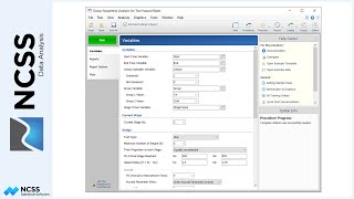
The Component, Data Column, and Type are specified for each of the 10 attributes. The desired estimation method is chosen. The percent error cutoff value defines which properties will be shown in the Poorly Estimated Properties Report. Running the procedure yields a series of numeric reports.
The first report displays summary information about the model estimation process. The second report shows the convergence of the nonlinear regression estimation process. The Differential Evolution Iteration Section displays the value of the criteria that is being minimized by the differential evolution algorithm. In this example, the criterion is the average absolute percent error between the actual and estimated sale price. The differential evolution search converged very quickly. Apparently, the nonlinear regression result was very close to or exactly the average absolute percent error estimate. The next report displays the details of the estimation of each parameter in the model. The Model Section displays the structure of the terms that make up each component. Here is the output form of this report.
Two Estimated Model Reports are given next. The first shows the model in reading form. The number of decimal places for the parameter estimates is set by the user. Here is how the model would look in documentation formula form. The second estimated model report gives the model with full precision parameter estimates. This expression may be copied onto the Clipboard and pasted into a transformation cell of the dataset to estimate other properties. This expression is always provided in double precision.
The Appraisal Ratio Section provides some of the basic statistics of an appraisal ratio study. For a much more comprehensive ratio study analysis, the estimated values should be stored in a column of the spreadsheet (using the Storage tab), and the Appraisal Ratio Studies procedure should be used.
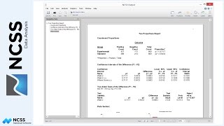
The next section shows the estimated sale price for all rows where the attribute data is given, but the sale price column value is left blank.
The next report shows the actual and estimated sale prices as well as 3 measures of disagreement. Assessors commonly study the ratio and/or the absolute percent error of estimated values to determine the quality or accuracy of appraisal.
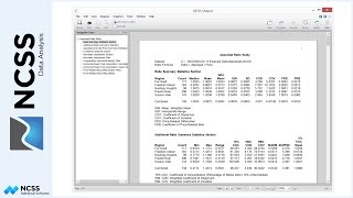
The Poorly Estimated Properties Section shows those rows with a large (percentage) difference from the estimated sale price to the actual sale price. The percent error cutoff, as set on the Reports tab, is 30%. Each row in this report should be analyzed to determine if there is some underlying explanation as to why the estimation is so poor. In some cases, it may be reasonable to try re-estimating the same model without these poorly estimated properties, to determine their influence.
Although no values were stored to the dataset in this example, the option is available to store the estimated values, residuals, or ratios to the spreadsheet. This is done by entering a column name or number on the Storage tab of the procedure and then running the procedure.
Determining the appropriateness of each model term is more difficult when using hybrid models as compared to multiple regression analysis. In multiple regression, the influence of each term may be measured directly, and even tested. In hybrid models, one can only look at the change in the minimization criteria when including or excluding a term. The tradeoff is flexibility. Hybrid models are more flexible.
Two statistics to consider when comparing hybrid model estimations are the final value of the minimized criteria (for example, Final Value of AAPE) and the R-squared value from nonlinear regression. When inclusion or exclusion of a term changes either of these values dramatically, it is likely an important term to include in the model.
Parameter estimates can also be monitored to determine if they make practical sense. For example, the plots tell us that the Glen Lake subdivision sale prices are generally much higher, and the Park Grove subdivision sale prices are lower. We would expect the parameter estimates to reflect this observation. In this example, the Glen Lake parameter estimate is 1.40, while the Park Grove parameter estimate is 0.86. These multipliers are consistent with the observed plots.
On the other hand, the pool coefficient estimate of 62,428 may be of concern, since it is such a large estimate, and only three properties were used in the estimation process. If the pool term is removed from the model, the model estimate changes from this… to this.
and the Final Value of AAPE changes from 11.72 to 12.17. The R-Squared changes from 0.880 to 0.871. Given this information, if $62,428 seems well outside the reasonable range for the effect of a pool, one may consider running the model without this term. The model should always be re-run when adding or removing a term. The change in all the other estimated parameters can be seen by comparing the estimated parameters of the before and after models.